(Needs proofreading! Written by: Dhruva)
About This Book
This is a place to store any and all resources and information relating to FRC Team 8726’s control subteam to provide a quick reference to all members and teach new members or members of other subteams some basics. You can quickly access this site anytime you need to on a laptop or phone at this URL.
Navigation
You can jump to different sections of the book using the sidebar on the left, and there is a search button in the top left you can use to search for words or phrases throughout the book.
There are also options on the top bar to change the theme and print the book (you can also save it as a PDF from there).
How was this made?
This book was created using mdBook, a tool for organizing markdown (.md) files into books which can also be hosted and navigated on a website. These files are hosted on GitHub - you can click on the GitHub logo in the top right to go to the repository. We use GitHub Pages to host the website.
It is the responsibility of the control subteam to keep this information up-to-date and document anything new. Feel free to reach out to a control member if you have any questions, or if you would like something added to this page. Or, better yet, add it yourself! For more information on doing this, see contributing.
Contributing
The GitHub repository containing all of the markdown files that make up this book and more can be found by clicking the GitHub icon in the top right. From there, you can make changes just like any other Git repository. If you are not familiar with Git, you may find it easier to use the web editor in GitHub, which should be sufficient for most purposes - just click the “Add File” button or click the edit button while viewing a specific file.
What’s in the repository?
An mdBook project contains a couple things.
- The
srcfolder contains all of the markdown files used to build this book. - The
themefolder contains overrides for the theme. The is only used right now to override thehighlight.jsfile. - The
book.tomlfile contains a few configuration options for the book as a whole. src/SUMMARY.mdis a special file which specifies how all of the pages are organized.
How to add or move pages
The src/SUMMARY.md file must be edited in order to add new chapter to the book or
change the ordering and organization of the chapters. The file looks something like this:
# Summary

- [Name of Chapter 1](path/to/page_1.md)
- [Name of Chapter 2](path/to/page_2.md)
  - [This is a sub-chapter](chapter/sub_chapter.md)
    - [You can go further too](source_file.md)
If you’re familiar with markdown, you probably recognize that this is just a bulleted list of links. (If not, don’t worry! It’s quite simple and there are some resources below to help you get started.) Simply add the name of the page you want to the list in brackets and then the path to the file in parantheses after in order to add another section.
Writing in markdown
Markdown (.md file extension) is a markup language used to style documents. You have likely already seen it in README.md files on GitHub, Discord messages, or somewhere else. It can do things such as bold or italicize text, add images, links, headings, code blocks, and more.
To get started, looking at a cheat sheet such as this one will show you how to format common things. Please do not write out code or equations in plain text.
Code can be written in short code blocks or longer ones like this:
void myFunction() {

}
The markdown syntax for that code block is:
```java
void myFunction() {

}
```
Additionally, mdBook supports several extensions to the markdown syntax which may be useful. The full list of supported extensions can be found in mdBook’s official documentation. Some of the supported features include tables and admonitions, which can be seen below:
| This is a | Table |
|---|---|
| Row 1 | Row 2 |
Note
This is an example of an admonition.
Adding equations
Rendering equations using LaTeX is supported in mdBook using MathJax.
This must be first enabled in the book.toml file, which has already been done.
If you are not familiar with LaTeX it looks a bit confusing but it uses backslashes to
insert special characters or functions into an equation. A cheat sheet can be found
here and a longer guide can be found
here (although it’s more in the
context of using LaTeX for a whole document).
Wrap inline equations in \\( \\) and equations that need their own line in \\[ \\]. For example, this:
\\( F_f = \mu \times F_N \\)
Looks like: \(F_f = \mu \times F_N \)
Linking to other parts of the documentation
Inserting hyperlinks in markdown is done using this syntax: [display text](https://example.com).
The same syntax is used to link to other parts of the book similar
to how you would link to other parts of a normal website. Instead of a URL,
use the local file path or the filename of the page you want to link to.
If you are linking to a page found in the same folder as the current page, then simply use the filename. Otherwise, you would need to cd back into the /src folder using ../ and then follow it up with the path to the destination (you may need to write ../ more than once).
For example, this page is located at src/about/contributing.md. If I wanted to provide a link to about.md,
which is found in the same folder, then I would write [about page](about.md).
If I wanted to link to the inventory page, which is found under /src/parts/, then I’d write [inventory page](../parts/inventory.md).
You can either use the markdown file ending (.md) or swap it out for .html, since an HTML file of the same name will be generated
when the book is built.
If you want to link to a specific section of a page, you can do that by adding
a ‘#’ after the file and then the name of the section, converted to kebab-case
with special characters like ‘.’ removed.
This is the same as the end of the URL you see in your browser when you visit
a certain page of the docs, so you can also just copy everything after the #
and use that to link to a specific section. For example, the link to this
section is https://cryptohawks8726.github.io/docs/about/contributing.html#linking-to-other-parts-of-the-documentation,
so to link to this section you would use contributing.html#linking-to-other-parts-of-the-documentation.
You can also use the full URL without the domain name, for example, /docs/about/contributing.html.
However, this will not work if the site is run locally or deployed somewhere other than /docs, so
it is recommended to use the local file paths instead.
Templates
The “List of Parts” and “FRC Software” chapters each have a file called “template.md” in their respective folders in the repository. When adding pages to these chapters you should copy the template and fill in the sections listed in the template to ensure you’ve covered everything. If a section of the template does not apply to the specific part or software it is recommended to specify that it does not apply instead of removing the section to avoid confusion.
What’s with highlight.js?
As mentioned earlier, the files in the theme folder overwrite
certain elements of the theme. The highlight.js file is responsible for syntax
highlighting in code blocks, and for some reason the default highlight.js file
only supports a small range of languages. It is notably missing support for Dart.
Because of this, it has been swapped out for a replacement file downloaded from the highlight.js library’s website which supports many more languages.
Building and Deploying
Anytime you make changes to the repository’s main branch, GitHub actions will automatically
rebuild the book and deploy it to the GitHub Pages site, so you do not need to do anything
manually for your changes to appear on the website. This is configured in .github/workflows/deploy.yml,
which has been copied from mdBook’s automated deployment examples.
This tells GitHub to run a few commands to build and then deploy the book to the site.
If you want to build the book locally to test it out, you can install mdBook’s command line tool
and run mdBook build, which will build a website in a folder titled book. Running mdbook serve will
host the website at localhost:3000. For more information and installation instructions,
see mdBook’s user guide.
Resources
Below are some helpful resources to reference when creating docs:
Important
Please don’t copy these verbatim. Only include information that is necessary and specific to our needs.
| Resource | Description |
|---|---|
| REV Documention | Provides information on different REV components/software (components are found in their own subcategories) |
List of Parts
Inventory
Mechanical keeps an inventory of parts on this spreadsheet.
Control keeps an inventory of their parts on this Google Doc (Requires an FCPS account to access).
These can also be found on the Schoology group under “Resources”.
Radio
This part can be found in {INSERT PLACE HERE E.G. CONTROL CABINET 1}
What is this?
Explain what this part does.
Ports
For the wire type, include the minimum/maximum wire gauge range (if there is one). Place a checkbox in the required column (or unfilled checkbox), as seen in this template. Follow the example seen in the table below.
| Port | Wire Type | Current Draw | Required | Where is it? | Additional Info |
|---|---|---|---|---|---|
| Example port | 11-13 gauge | 7000000 amps | ✓ | next to the green light | this port will explode |
| Other port | 67 gauge | 92813789 amps | ✗ | inside the stomach | this port may explode |
Status Lights
Does this part have any status indicators? If so, list them. Feel free to remove this section for parts that obviously do not have status lights.
Software Updating
Does this part need software updates? If so, how? Feel free to remove this section for parts that obviously do not have software.
Extra information
Add any extra information here, or remove this section.
Official Documentation and Manuals
Put links to anywhere containing more info about the part here. You can put a link to a store where we can buy the part here too.
ismail - not proofread nor complete
SparkMax
Can be found in the mechanical room on the gray shelves (not to be confused with the toolcarts). They will be in a bin labeled “Spark Max”.
Overview
Sparkmaxes are the motor controllers of choice for 8726, at least for our REV motors. They can be configured, analyzed, and controlled via a USB connection using REV Hardware Client.
Ports
| Port | Wire Type | Current Draw | Required | Where is it? | Additional Info |
|---|---|---|---|---|---|
| CAN port | Custum REV Spark Max CAN Adapter - 22 AWG | amps | ✓ | Side connecting to PDH, next to USB-C port | Used to connect to the CAN bus |
| 6-pin Encoder port | 6 x 24 AWG Encoder Wire | amps | ✓ | Side connecting to motor | Enables connection to the motor’s encoder |
| USB-C port | USB-C cable | -? amps | ✗ | Side connecting to PDH, next to CAN port | Used to connect to [REV Hardware Client] (../software/rhc.md) |
| PDH Power Wire port | 2 x 12 AWG Power wire | ? amps | ✓ | Side connecting to PDH | Used to power the SparkMax and the Motor it is controlling |
| Motor-Side Power Port | 3 x (14 iirc maybe 12) AWG Power wire | ? amps | ✓ |
Status Lights
ismail - not proofread nor complete
REV motors
The two REV motors we use are apart of the REV ION Brushless package.
NEO
NEOs are compact and lightweight brushless motors.
NEO Vortex
A NEO Vortex (Vortex for short) is essentially an upgraded version of a regular NEO, designed for high-power applications.
NEO Vortexes are typically controlled using a SparkFlex motor controller. SparkFlexes are mounted directly onto Vortexes; they contain most of the key features found in SparkMaxes along with a few additions. 8726 does not use SparkFlexes, however. Instead, a special Solo Adapter has been mounted in place for Sparkmaxes to connect to.
| Port | Wire Type | Current Draw | Required | Where is it? | Additional Info |
|---|---|---|---|---|---|
| 6-pin Encoder port | 22 gauge | amps | ✓ | Side connecting to motor controller | Enables connection to the motor’s encoder |
(Needs proofreading! Written by: Keshav)
RoboRIO
This part can be found in Control Cabinet 1.
What is this?
The roboRIO is the robot’s main controller. It runs the robot program we deploy with WPILib Java, communicates with the Driver Station, and connects the code to sensors and motor controllers. Commands and subsystems execute on the roboRIO, while motor controllers do the high-current work of driving the motors. The roboRIO is therefore a control computer, not a replacement for a PDP/PDH or a motor controller.
Ports
| Port | Wire type | Required | Where is it? | Additional info |
|---|---|---|---|---|
| Power input | Uh red and black power wires | ✓ | Power connector on the roboRIO | Connect to the PDP/H. Verify polarity before powering on. |
| Ethernet | Standard Ethernet cable | ✓ | Ethernet jack | Wired to the robot radio |
| USB device (Type-B) | USB Type-B cable | ✗ | USB device jack | Used to connect a computer for roboRIO imaging |
| CAN bus | CAN-H/CAN-L twisted pair using the team’s approved CAN wiring | ✓ | CAN connector | Connects CAN motor controllers and sensors. Keep CAN-H and CAN-L paired, observe polarity, and terminate the bus correctly. |
| A whole lot of others | Varies - there is multiple types | ✗ | Everywhere | We never use these and they are very old. They are for older moters which don’t use the CAN protocol but we use modern motors which support CAN |
Status Lights
The LEDs are useful for diagnosing a robot before opening the code. The roboRIO status-light meanings are:
| Light | Normal meaning | If it is not normal |
|---|---|---|
| Power | Green: power is good. | Amber indicates brownout protection; red indicates a power fault or user-rail problem. Check robot power, connectors, and wiring. |
| Status | Off after a normal boot. | Two blinks indicate a software error; three blinks indicate Safe Mode; four blinks indicate repeated software crashes. Reboot and reimage if the problem remains. |
| Comm | Solid green: good Driver Station communication. | Off means no communication; solid red means the Driver Station is connected but user code is not running; blinking red means E-stop. |
| Mode | Off when outputs are disabled, orange in autonomous, green in teleoperated, and red in test. | A mode that does not match the Driver Station usually indicates a communication or enable-state issue. |
Use the WPILib status light quick reference for the complete list. Do not repeatedly enable a robot while a power or software fault is present.
Software Updating
The RIO Firmware has to be manually updated every season using the RIO Imaging Tool.
Official Documentation and Manuals
- WPILib: Imaging a roboRIO 1
- WPILib: Imaging a roboRIO 2
- WPILib: Status light quick reference
- WPILib: Recovering a roboRIO using Safe Mode
- WPILib: FRC Game Tools
- Our RoboRIO Imaging Tool page
Batteries
Batteries can be found in the electrical room, stored in the battery charging station. Charged batteries are labeled and kept separate from depleted ones.
What is this?
The FRC robot battery is a MK ES17-12 12V 18Ah Sealed Lead Acid (SLA) battery. It is the sole power source for the entire robot, supplying 12V DC to the Power Distribution Hub (PDH), which then distributes power to all motors, sensors, and control system components. Each match, the robot runs on a single battery. Teams typically rotate through multiple batteries between matches to ensure full charge.
Ports / Connections
| Port | Wire Type | Current Draw | Required | Where is it? | Additional Info |
|---|---|---|---|---|---|
| Positive terminal (+) | 6 AWG copper, red/yellow/white/brown or black w/ stripe | Up to 270A peak (5s) | ✓ | Top of battery, bolt terminal (M5) | Must use ring terminal; connects to red battery cable leading to main breaker |
| Negative terminal (−) | 6 AWG copper, black or blue | Up to 270A peak (5s) | ✓ | Top of battery, bolt terminal (M5) | Must use ring terminal; connects to black battery cable leading to main breaker |
| Anderson SB50 Connector | 6 AWG copper, red and black | — | ✓ | End of battery cable assembly | Mates with robot-side SB50 connector; gray and black housings are intermateable, use consistent color |
Note: Per the FRC Game Manual, battery leads must be copper, minimum 6 AWG (16 mm²), maximum 12“ long, color-coded for polarity.
Extra Information
- Voltage: 12V nominal; 12.7–13.5V open circuit when fully charged
- Capacity: 18 Ah (20-hour rate)
- Weight: ~12.89 lbs (5.86 kg)
- Dimensions: 7.13“ × 2.99“ × 6.57“ (181 × 76 × 167 mm)
- Max discharge current (5s): 270A
- Internal resistance: ~12 mΩ (ideal: <15 mΩ; replace if >20 mΩ)
- Charger settings: Cycle use 14.4–15.0V; max charge current 5.4A
- Case material: ABS (UL94 HB flame retardant)
- Batteries should be checked with a battery beak or similar tool before each match. A fully charged battery should read above 12.5V under load.
- Never leave a battery fully discharged for extended periods — this degrades SLA batteries significantly.
- Do not use non-SLA or lithium batteries; they are not FRC-legal.
Official Documentation and Manuals
- WPILib Robot Battery Basics
- MK ES17-12 Datasheet (PDF)
- AndyMark Battery Listing
- FRC Game Manual — R601 (Battery Rules)
SystemCore
Ismail
PDH/PDP and Fuses
Kraken X60
Playing sounds
- ismail, not proofread
Wagos
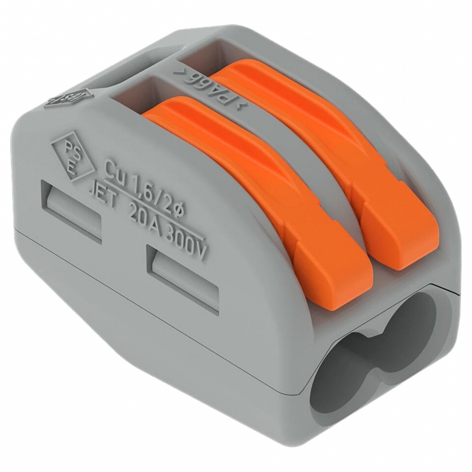
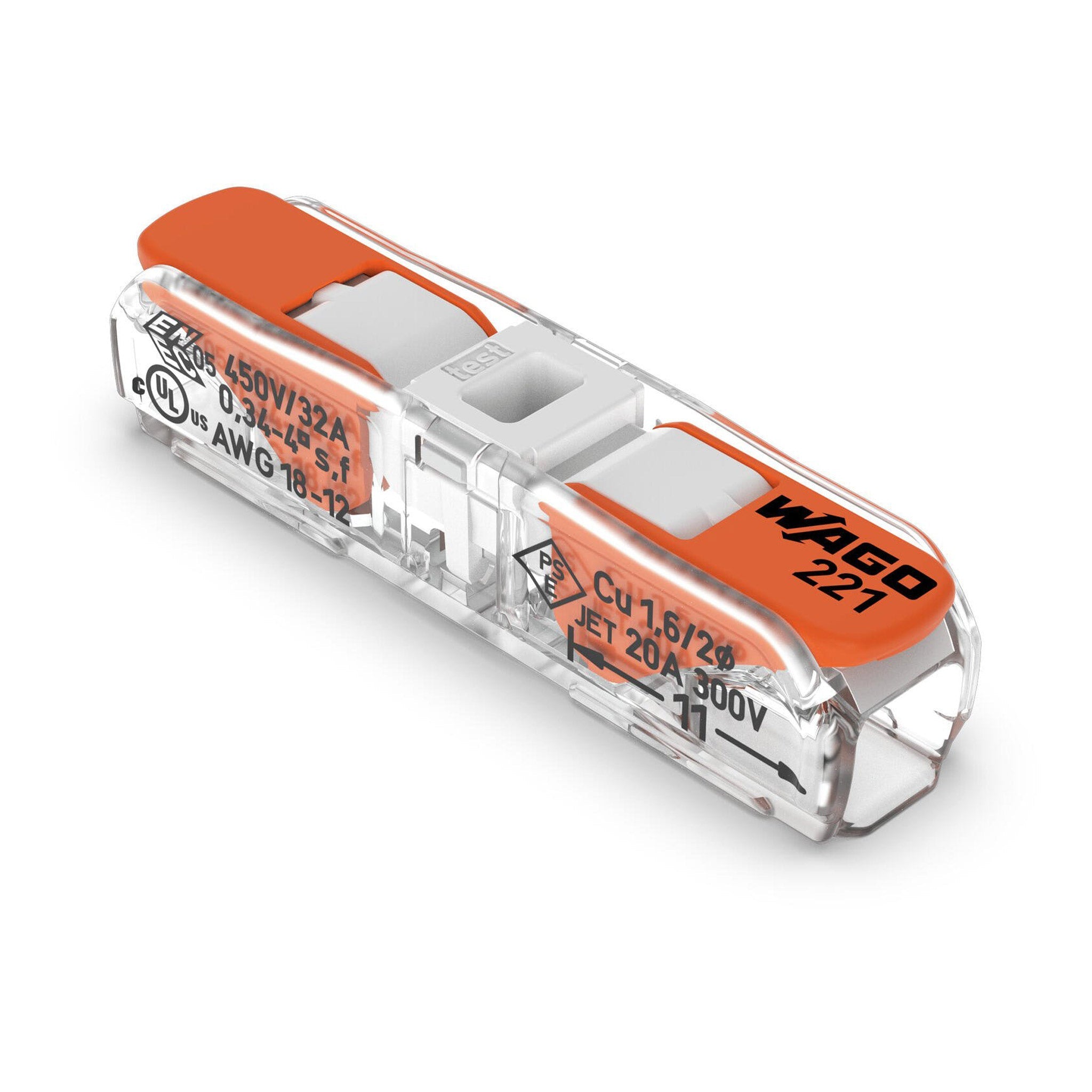
This part can be found in the Mechroom inside the electrical bin.
What is this?
WAGOs are wire connectors that allow wires to splice together without the need to sauder or use screws. Using them, wires can easily secure in place and be interchanged when needed.
8726 mainly uses 2 types of WAGOs. Gray WAGOs (Image 1) are used to connect wires with a guage of at least 28 AWG (i.e CAN and Encoder wires). Clear WAGOs with orange tops (Image 2) are usually used to connect power wires; they may also be used to connect high-guage wires if we run out of gray WAGOs.
Common issues
The following are some common issues that may arise when using WAGOs, along with some solutions.
| Problem | Solution |
|---|---|
| Wires come off easily with little force. | Ensure that the wire is stripped enough, restrip the wire if need be. |
| Connection not working or wires not being powered | Make sure that the wire is not frayed or missing strips. You may need to either restrip the wire or use a different one entirely. |
| Wires don’t fit | Make sure that the WAGO being used is of the correct gauge. Restrip the wire if it is not stripped properly. |
Tools
Jacob
VRM
Ron
ismail - not proofread
RSL
This part can be found in Control Cabinet 2
What is this?
The RSL is a large LED light used to determine the current status of the robot; it is mandatory for competition.
Ports
| Port | Wire Type | Current Draw | Required | Where is it? | Additional Info |
|---|---|---|---|---|---|
| La | 22 gauge | 60 miliamps | ✓ | Bottom of RSL | Positive Terminal |
| N | 22 gauge | 60 miliamps | ✓ | Bottom of RSL | Negative Terminal |
| Lb | 22 gauge | 60 miliamps | ✓ | Bottom of RSL | Positive Terminal |
The RSL has 3 power ports. The middle port is for the negative terminal (black wire). The two outer ports are for the positive terminal (red wires).
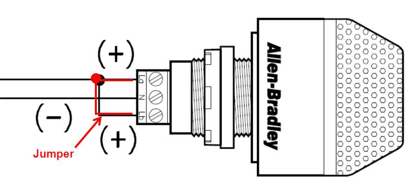
Run the main red wire through La, then connect La and Lb with a separate red wire that will act as a jumper cable. Connect La to S and N to Ground on the roboRIO.
Status Lights
The robot’s status is determined by 3 different modes:
| Mode | Meaning |
|---|---|
| ON and SOLID | Robot is on and disabled |
| ON and BLINKING | Robot is on and enabled |
| OFF | Robot is off, RSL not wired properly |
Official Documentation and Manuals
- ismail - not proofread nor complete
Pigeon
This part can be found in Control Cabinet 1
What is this?
The CTRE Pigeon is an IMU (Inertial Measure Unit) commonly used by many FRC teams to measure odometry.
Cameras and Limelights
120A Main Circuit Breaker
The main breaker can be found mounted on the robot, typically on the outside of the frame perimeter in an accessible location. It must be easily reachable and operable by a referee or field staff at all times during competition.
What is this?
The Eaton Bussmann CB285-120 is the FRC-legal 120-amp main circuit breaker required on every FRC robot. It serves as the master power switch and overcurrent protection device for the entire robot. It connects in-line between the battery and the Power Distribution Hub (PDH), and can be used to manually cut all robot power in an emergency. It is a Type III (switchable/manual reset) thermally responsive breaker — it can trip automatically under sustained overcurrent, or be manually switched off.
Per the FRC Game Manual, this specific breaker (CB285-120) is the only legal main breaker for FRC competition robots.
Ports / Connections
| Port | Wire Type | Current Draw | Required | Where is it? | Additional Info |
|---|---|---|---|---|---|
| Battery-side stud (input) | 6 AWG copper, red (positive) | Up to 120A continuous | ✓ | One of two M6 terminal studs | Connects from the Anderson SB50 robot-side connector; ring terminal required |
| PDH-side stud (output) | 6 AWG copper, red (positive) | Up to 120A continuous | ✓ | Second M6 terminal stud | Connects to the PDH positive input terminal; ring terminal required |
Note: Only the positive (red) wire passes through the main breaker. The negative (black/blue) wire runs directly from the battery cable to the PDH negative terminal, unbroken.
Status Lights
The CB285-120 does not have a status LED. Instead, it has a visible yellow reset lever that shows the open (tripped) condition. When the breaker is tripped:
- The yellow lever will be in the raised/protruding position.
- Push the lever back in to reset the breaker (only after resolving the cause of the trip).
The breaker also has a red push-to-trip button that can be used to manually cut power.
Extra Information
- Manufacturer: Eaton Bussmann
- Part Number: CB285-120
- Rating: 120A, 6–48V DC
- Interrupt rating: 3 kAIC
- Type: Type III — switchable, manual reset, trip-free
- Terminal: M6 stud (accepts 1/4“ ring terminals)
- Operating temperature: -40°C to 85°C
- Size: 2.9“ × 1.9“ × 1.5“ (73.7 × 48.3 × 38.1 mm)
- Weight: 0.24 lbs
- IP Rating: IP67 (weather resistant / waterproof housing)
- The breaker is “trip-free” — it cannot be held closed after it trips. Do not attempt to force it closed during a trip.
- The breaker must be easily accessible on the robot; FRC rules require that a referee can cut robot power quickly.
- Do not substitute with any other breaker — only the CB285-120 is FRC-legal as the main breaker.
Official Documentation and Manuals
- WPILib Wiring Guide (Main Breaker)
- AndyMark CB285-120 Listing
- CTR Electronics CB285-120 Listing
- Eaton CB285-120 Product Page
- FRC Game Manual — R609 (Main Breaker Rules)
Encoders
CANCoders
FRC Software
Ronith
(Needs proofreading! Written by: Dhruva)
Visual Studio Code
We may use two different versions of Visual Studio Code:
- WPILib’s custom build of VS Code with FRC-related features.
- The regular version of VS Code, for use with non-robot code projects
Where to download/update
WPILib’s custom build: With the rest of WPILib
Regular version: https://code.visualstudio.com/download
The regular version of VS Code will update automatically. WPILib’s build will update when you install new versions of WPILib.
For more information on installing and updating WPILib and its tools see the WPILib page
Description
VS Code is a text editor with support for extensions and utilities to run and debug code.
How to use
- Building and deploying robot code: See the guide on robot code deployment
- Open file: Go to “File” on the top bar and click “Open Folder”, then select the folder.
- Install extensions: Go to the extensions page on the sidebar and search for the desired extensions.
- Creating WPILib projects: See WPILib’s docs
Official Resources
FIRST Driver Station (written by Ron, needs proofing)
Where to download/update
Download: FIRSTDriverStation
Linked above is the official download link of the FirstDriverStation, this application needs to be updated manually (As of August 1st 2026). Download the version that matches your operating system and processing unit, it is listed on the GitHub release page below.
Description
Driver Station is the main control panel for your FRC Robot. It manages your Teleoperated, and Autonomous routines during practice. The Driver Station acts as a communicator between your controller and the robot. As well, this is the station you will use during the 2 Match Weeks you have during the season, by connecting to the Ethernet provided behind the glass.
How to use

Above is the updated version of Driver Station for the 2027 FRC season, this is the main control panel you will see when testing the robot, and competing during the competition. We will go through what each part means in the station.
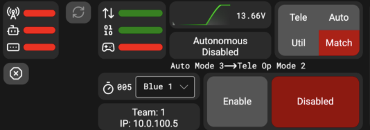
The main control panel is shown above. In the top left we can see the connectivity with the robot and the FMS station. On the right, we can see the connectivity between the Robot marked by the arrows, we can see the robot code marked by the 0110, and the controller connectivity marked by the controller, before we start a match or a practice we want to see all greens on the panel. Below this connectivity panel we can select which team we are, Red/Blue (1-3). As well we see a graph of the battery voltage, during matches and practices we always want to see this over 12V, anything below 12V means that we are “browning out” which means we need a battery switch. Below the battery voltage we can see the status of the robot whether we are in Auto or Teleop, and whether we are Enabled or Disabled, make sure the robot is disabled every time you are not running the robot. On the top right, we can choose between Teleoperated, Autonomous, Match, and Utilities, changing these modes depending on the type of testing you are doing. When this program gets updated, you will be able to see match timers when you run the robot.
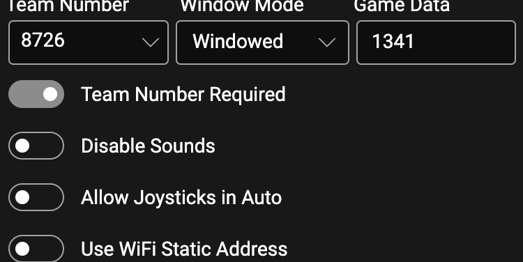
Above we can see the beginning part of the settings, we can see the Team Number (always keep this on 8726, unless you’re not 8726 :P). Keep the Window Mode to DOCKED as Aluminum (our team’s custom Driver Dashboard) will fit to it. Use the Game Data value set to send data to our robot.
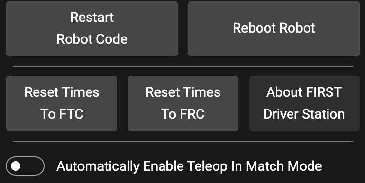
When we scroll down to this part, make sure that you reset the Robot Code anytime you update or pull code from GitHub. Then make sure that you always reset times to the FRC standard (because we are in FRC :D). Leave everything unchecked unless necessary or directed to do so. Official Resources
Resources
Linked below are some resources to aid your journey, if more help is necessary, ask the Driver, Operator, or Technician. Have fun!
Choreo and PathPlanner
Go to the Autonomous Folder for more in-depth documentation on Choreo and Pathplanner
What is Choreo?
Choreo stands for: Constraint-Honoring Omnidirectional Route Editor and Optimizer. Choreo allows FRC teams to design drivetrain paths on custom maps that run during the autonomous period in a game. The autonomous period is one of the most important periods in a match. Depending on the game, it can provide benefits such as ranking points, point advantages, and an overall better position when the teleoperated period starts.
Choreo allows:
- The creation of drivetrain paths
- Implementation of commands into autonomous paths
- Creating the paths on top of a custom game field
- Splitting paths into multiple sections
- Implements with Pathplanner for better command control
- Path preview
- The creation of custom events
Link to Choreo: https://choreo.autos/
What is Pathplanner?
Pathplanner is a tool very similar to Choreo and can do most of what Choreo does. At CryptoHawks(The BEST team), we use it to order sections of paths, order commands, and run certain things in parallel or sequential. Pathplanner also allows for custom game fields to be added and can have Choreo paths imported into it.
Pathplanner allows:
- Path preview
- Creation of event markers
- Creating sequential and parallel command groups
- Ordering of commands
- Importing Choreo paths
Link to Pathplanner: https://pathplanner.dev/home.html
Phoenix Tuner X
Kabir
REV Hardware Client
Kabir
(Needs proofreading! Written by: Dhruva)
Aluminum
Where to download/update
Aluminum is maintained by our team.
Downloads:
Public version: [Link TODO]
8726 private version: [Link TODO]
To update Aluminum download the latest release and run the installer. Make sure it is up to date on the driver laptops before matches!
Description
Aluminum is an app made by our team to function as a dashboard for drivers and provide several utilities for debugging robots, as well as running tests for prototypes.
How to use
Navigating the app: See this page.
Running prototypes with MotorTester: See this page.
Official Resources
These docs, as well as the README files in Aluminum’s GitHub repo, are the only official resources on Aluminum, as it is maintained by our team.
RoboRIO Imaging Tool
Ismail
(Needs proofreading! Written by: Dhruva)
GitHub Desktop
Where to download/update
Download: https://desktop.github.com/download/
Downloaded as a windows installer.
GitHub desktop will update automatically once installed.
Description
GitHub desktop is an application to run commit git tasks like pushing to/pulling from a repository, cloning repositories, and managing cloned repositories. It is an alternative to the Git CLI.
How to use
For more information on using GitHub Desktop see the Git and GitHub section of the docs.
Official Resources
Documentation: https://docs.github.com/en/desktop
More help can also be found in the application by clicking “Help” at the top bar.
WPILib Tools (Glass, SysID, etc)
Glass
Jathon
GrappleHook
Jacob
(Needs proofreading! Written by: Keshav)
Limelight Hardware Manager
Where to download/update
Download: Official Limelight Downloads
Download the version that matches the computer’s operating system and processor. On Linux, the program is distributed as an AppImage and may need to be marked as executable before it can run.
The Hardware Manager does not automatically update itself. Check the official downloads page for a newer version, especially before flashing a Limelight or configuring Limelight.
LimelightOS is also updated manually. The Hardware Manager and LimelightOS are separate:
- Limelight Hardware Manager runs on the programmer’s computer.
- LimelightOS runs on the Limelight camera.
Installing a new Hardware Manager does not update the camera. The correct LimelightOS image must be downloaded and flashed separately.
Important
Limelight provides different OS images for different hardware models. Verify whether the camera is a Limelight 1/2/2+, Limelight 3, Limelight 3G, Limelight 3A, or Limelight 4 before downloading an image. Flashing should follow the quick-start instructions for that exact model.
Description
Limelight Hardware Manager is the desktop utility used to find and maintain Limelight cameras. Its two main jobs are:
- Discover Limelights connected to the same network and open their configuration pages.
- Flash a Limelight with a new LimelightOS image over USB.
The Manager also displays useful discovery and network information, making it easier to determine which cameras are connected and how to reach them.
The Hardware Manager is not where most Limelight configuration happens. Double-clicking a discovered device opens the camera’s built-in web interface. That browser interface is where we configure:
- Team number
- Hostname
- Static IP address
- Camera position on the robot
- AprilTag field map
- Vision pipelines
- Exposure, gain, resolution, and frame rate
- Crosshair and targeting settings
- LED and stream settings
Those settings are hosted by the Limelight itself and are saved to the camera.
How to use
Find a Limelight on the robot network
- Power the Limelight and connect it to the robot radio with Ethernet.
- Connect the programming laptop to the robot’s network.
- Open Limelight Hardware Manager.
- Select Scan.
- Wait for the camera to appear in the device list.
- Double-click the camera to open its web interface.
A Limelight with the default hostname may also be opened directly at:
http://limelight.local
If a static IP has already been assigned, it can be opened with:
http://<limelight-ip>
(If it says not found or something put :5801 at the end of the url)
The Hardware Manager is especially useful when we do not know the camera’s hostname or IP address.
Configure a new Limelight for Team 8726
After opening the camera’s web interface, go to the Settings tab.
Set the team number
Set the FRC team number to:
8726
The team number is required for the Limelight to connect to the correct NetworkTables server.
Set a hostname
One Limelight can use the normal limelight hostname. If the robot has multiple Limelights, every camera must have a unique hostname.
Use descriptive names based on physical location or purpose:
limelight-front
limelight-back
limelight-left
limelight-right
The hostname is also used by LimelightHelpers and NetworkTables, so code must use the same name.
Open the web interface without Hardware Manager
Hardware Manager is convenient, but it is not required every time. Once networking is configured, open the camera directly from a browser using its hostname or static IP.
The web interface provides:
- Settings: network, team number, hostname, and system configuration
- Pipeline tabs: AprilTag, color, neural-network, Python, and other vision pipelines
- Camera and Crosshair: exposure, gain, resolution, orientation, LED, and targeting calibration
- 3D Visualizer: AprilTag detections and field-space localization
Changes made in the web interface are saved automatically by LimelightOS. Even so, important pipelines should be backed up before major changes.
Update LimelightOS
Use the instructions for the exact Limelight model. The general process for current Hardware Manager releases is:
- Back up pipelines, scripts, and important settings.
- Power off the Limelight.
- Download the newest Hardware Manager.
- Download the newest compatible LimelightOS image for the camera model.
- Connect the Limelight directly to the laptop using a USB data cable.
- Put the camera into flash mode as described by its official quick-start guide.
- Open Hardware Manager and select the Flash OS tab.
- Select the downloaded OS image and wait for it to extract.
- Select Refresh Device List.
- Select the Limelight flash device.
- Select Flash Device.
- Wait for flashing to finish before disconnecting the camera.
- Remove USB, reconnect normal robot power and Ethernet, and allow the camera to boot.
- Restore and verify its network settings, camera pose, pipelines, scripts, and calibration.
Some models enter flash mode as soon as USB is connected, while others require holding the configuration button while connecting USB. Follow the model-specific guide instead of guessing.
Use a USB cable that supports data, not a charge-only cable. Do not disconnect the camera or close the program while flashing.
Verify the update
After flashing:
- Scan for the Limelight with Hardware Manager.
- Open its web interface.
- Confirm the reported LimelightOS version.
- Verify the team number, hostname, and static IP.
- Restore pipelines and scripts if necessary.
- Confirm the correct FRC field map is installed.
- Confirm the camera pose relative to the robot.
- Verify NetworkTables communication.
- Test every pipeline used by robot code.
- Test localization with real field AprilTags before competition.
A successful flash only proves that LimelightOS was installed. It does not prove that the camera is configured correctly for the robot.
Configure multiple Limelights
Every camera must have:
- A unique hostname
- A unique static IP
- The correct team number
- A camera pose matching its real location and orientation
For example:
| Camera | Hostname | Static IP |
|---|---|---|
| Front | limelight-front | 10.87.26.11 |
| Back | limelight-back | 10.87.26.12 |
Robot code must request results from the correct hostname:
Do not leave multiple cameras with the default hostname or the same IP address. That creates discovery and NetworkTables conflicts.
Troubleshoot a Limelight that does not appear
Work through the connection from the bottom upward.
Check power and wiring
- Confirm the Limelight is powered.
- Check its status lights.
- Confirm Ethernet link lights are active.
- Reseat the Ethernet cable.
- Confirm the laptop is connected to the same robot network.
- Try a known-good Ethernet cable.
Scan again
- Close and reopen Hardware Manager.
- Select Scan again.
- Allow the Limelight enough time to boot.
- Temporarily disable unrelated network adapters or VPNs if they interfere with discovery.
Try direct access
Try:
http://limelight.local
and the last known static IP.
For Limelight models that support USB networking, connect with USB and use the address listed in that model’s quick-start guide.
Check hostname resolution
If the static IP works but the .local hostname does not, the camera is reachable and name resolution is the problem. Older Windows installations may require Bonjour, which is available from the Limelight downloads page.
Check network configuration
An incorrect static IP can place the Limelight on another subnet. Use Hardware Manager discovery, a supported USB-network connection, or the model’s documented network-reset procedure to recover it.
Do not flash LimelightOS merely because the browser cannot find the camera. First verify power, Ethernet, laptop networking, hostname resolution, and IP configuration.
The Limelight does not appear in the Flash OS tab
- Confirm the USB cable supports data.
- Connect directly to the laptop instead of through a hub.
- Follow the correct button procedure for that Limelight model.
- Wait for the computer to enumerate the flash device.
- Install the official USB/RPIBoot driver when required.
- Select Refresh Device List again.
If the device still does not appear, follow the model-specific flashing instructions on the official quick-start page.
When to use Hardware Manager
Use Hardware Manager when:
- Setting up a new Limelight
- Finding a camera with an unknown IP address
- Opening the web interface
- Diagnosing which Limelights are visible
- Updating or recovering LimelightOS
You normally do not need it open while programming or operating the robot. Once configured, the Limelight communicates with robot code and dashboards over the robot network.
Official Resources
- Limelight Downloads
- Limelight Documentation
- Limelight 2/2+ Quick-Start
- Limelight 3 Quick-Start
- Limelight 3G Quick-Start
- Limelight 4 Quick-Start
- Limelight APIs and Libraries
(Needs proofreading, should we add anything else here? Written by: Dhruva)
Our Projects
This chapter contains in-depth information about some of our projects besides our robots themselves. You can find guides on what they are, how they are meant to be used, and information to help maintain them in the future.
(Needs proofreading! Written by: Dhruva)
Aluminum
Aluminum is an app made by the team. It should be kept up to date on all team laptops. If it is not installed or is out of date, please let someone know or update it yourself.
Aluminum has a variety of utilities and may have more features added in the future. It can communicate with robots through NetworkTables, allowing the app to observe and change data sent from the robot. It can also connect to a simulated robot.
The app will switch between red and blue themes depending on the robot’s current alliance.
Using Aluminum
Aluminum will open to the dashboard screen, with a field view and information displays that would be useful to a driver during matches. To get to other parts of the app, click on the logo in the bottom right and select a page to go to. The auto selector is also located here, which is used to set the auto routine the robot will run if it is activated in the autonomous period. You can find the version number at the bottom of this panel.
Above the logo button is an expand button. Clicking on this will toggle between the window being docked above the driver station window. When the driver station is open (preferably in its docked mode at the bottom of the screen) and this button is clicked, the app will automatically resize itself to take up all of the remaining screen area above the driver station and the window bar above it will disappear. Clicking the button again returns the window to its normal state.
Settings
Aluminum has some settings you may need to change. Settings can also be saved to a JSON file and loaded onto another computer if needed.
Important
Make sure to click the “Save Changes” button in the top right after making any changes!
Aluminum has several settings which must be set correctly to connect to the robot. The default settings should work for a real robot. The team number and port must be set correctly - the default port used for NetworkTables is 5810, and our team number is (obviously) 8726. If the “Use server name instead of team number when connecting” option is enabled, instead of attempting to connect to 10.TE.AM.1:PORT, the app will attempt to connect to the specified port at whatever address you put in the server name field. This can be used to connect to a simulated robot by connecting to “localhost”.
Cameras are also configured from settings. Aluminum can display any number of MJPEG streams on the dashboard screen. The IP address of each stream must be set to the correct IP or you will not see anything on the dashboard. See the page on cameras for more information about where to find these IPs.
The Dashboard
The dashboard is the first screen you see in Aluminum and has several pieces of information. The live feed from any connected cameras is shown on the left. On the right, you can find the match number, game timer, and alliance. There is also a field view, which shows the robot’s position on the field and has a button to reset the robot’s gyro if needed. Information about the robot’s current state and specific values can be displayed below. Finally, there is a network connection indicator in the bottom right which will turn green if connected to a robot.
The Debug Panel
Aluminum’s debug panel functions similarly to Glass, although it can be more convenient since it is organized to work with how our team typically structures data in NetworkTables, allowing you to easily view data for each individual subsystem.
Testing Motors
Aluminum provides an interface to make working with the MotorTester code easier. For more information on this feature see the section on MotorTester.
(Needs proofreading! Written by: Dhruva)
Codebase Overview
Aluminum is built using the Flutter framework, a framework made by Google for building modern cross-platform GUI apps. We only target Windows currently, but the app has been shown to build successfully on MacOS and Linux and would likely be usable on other platforms as well.
Aluminum is currently split into several branches to keep game-specific code isolated, since we may add specific displays to the dashboard or other changes which are only useful for one season. A basic template and any utilities which should be shared across different games should be kept on the main branch. Separate branches are created for the specific configurations used for each game (e.g. 2026-main).
About Flutter
Flutter uses Dart as its primary scripting language, although it uses a C++ engine on the
backend. Dart is similar to Java as it is also run inside a virtual machine and compiles
to bytecode (well sort of, usually… see here for more info),
although it has more modern syntax features such as
null safety, optional support
for dynamic types, and is organized by “libraries” instead of classes, allowing you to
have functions or variables which are not associated with a class for more functional
programming. Dart also has better type inference—while Java allows you to declare local
variables with var, it is not very commonly used. In Dart, you will often see variables
declared with only var or final and the compiler will infer the variable’s type. Dart
has similar object-oriented features, although it does not have explicit public or private
modifiers, however, prefixing a class or function with an underscore will make it inaccessible
outside of the current library.
For help getting started with Flutter, you should look at the official docs, where there are beginner tutorials, videos, API docs for the full library, and more.
Building apps with Flutter requires the Flutter SDK to be installed, which comes with a command-line tool for building and running Flutter projects. As of right now, this is only installed on Laptop #8 but this may change in the future. There is also a VS Code extension for running flutter directly from VS Code. A guide to installing the SDK can be found here in official documentation.
NTCore Bindings and FFIGen
This project uses Dart FFI (Foreign Function Interface) bindings to interface with the NTCore library, part of WPILib. This library has a C API which can easily be called from other languages, like Dart. Dart bindings were automatically generated using the ffigen package, creating lib/ntcore/ntcore.g.dart. The main app code shouldn’t directly use these bindings—instead, go through the classes provided in lib/ntcore/instance.dart, which have all been documented and have methods which can safely and easily be called from dart without interacting with native memory. You can easily add extra methods to NTInstance or create another class if you need to access other parts of the C library which do not currently have safe dart bindings written for them.
In order to regenerate the bindings, run tool/ffigen.dart (dart run tool/ffigen.dart). You may need to provide the location
of the C standard library headers, which it for some reason can’t find sometimes (linux error, no clue if this happens on windows :P ),
so locate wherever those headers are on your
system and set your CPATH environment variable to that or temporarily add it to the compiler arguments in tool/ffigen.dart.
You may need to update the bindings if WPILib changes or adds to the NTCore C API. To do this, download the headers (the easiest place to get them is wpilib’s maven releases. Go to the ntcoreffi releases, where there is a .zip file containing all the headers. Unzip all the NTCore headers into ntcore_headers/include, replacing the old files. Then, follow the above instructions to regenerate the bindings, and make sure there are no new errors and implement any new functionality.
Dart bindings for NTCore have been made in lib/ntcore, which contain several classes and methods to perform
common functions without having to directly interface with native functions and handle things like memory
allocation. lib/ntcore/instance.dart contains the NTInstance and NTValueNotifier classes which handle most of
this functionality. lib/ntcore/library_link.dart contains code necessary to load NTCore at startup and
lib/ntcore/values.dart contains the NTValue class, which is a sealed class
that can be used to handle the different types of values in NetworkTables.
NTCore uses pointers to the WPI_String struct for strings. You can convert to/from dart strings using toWpiString and wpiToDartString methods. If you don’t have a pointer to a WPI_String struct you can also cast the str field to a Utf8 pointer and then call toDartString() with the length from the len field.
Using the NTCore Bindings from Dart
The app should make a single instance of NTInstance (ntcore/instance.dart), which is the main class responsible for communication with NetworkTables. Then, use updateConnectionSettings or updateServerNamePort to connect to a specific NT server. You can either connect to the rio via team number and port 5810, or to a sim using localhost:5810. The NTInstance will then keep track of any entry handles in use to publish/subscribe to avoid memory leaks and keep publishers alive.
The NetworkTablesValue class is a sealed class with subclasses for each value type in NT. You can use a switch statement to check what type a value is or use an if statement to check if it matches a certain type. Also, the toString method will return an appropriate string representation of the value, whatever type it is.
The NTValueNotifier class is used to provide a ChangeNotifierProvider object which notifies listeners any time the value at a certain path in NetworkTables changes. Internally, NTInstance polls listeners and updates them in a loop, and this is how these updates are handed out. The easiest way to create new NTValueNotifiers is to use the .fromName factory, which either creates a new one or returns an existing listener for that entry. We keep most of the paths and notifiers (and the NTInstance) used as global variables in one file (lib/ntreferences.dart). There is also an NTPrefixNotifier class which tracks a map of all the values under a certain prefix.
Where to find specific things
- lib/screens contains files for each one of the screens on the dashboard - the main dash, settings, motor tester panel, etc. Each just has a class extending Widget which contains all the logic for that screen.
- lib/widgets contains some specific widgets used such as the field view widget and the auto chooser widget.
- main.dart is the entry point and has the main app and scaffold as well as the side drawer. It also maintains a list of all the screens, labels, and icons for each one - if you’re adding a new screen make sure to add it to that list.
- util.dart contains some random things
- settings.dart contains the logic for saving, loading, and accessing settings to/from json files.
The settings system
This system is contained entirely inside lib/settings.dart.
Settings are stored in a settings.json file in the app’s config directory (the appropriate
directory for the current platform is fetched by the app_dirs package). This is loaded into
the Settings class at startup inside an instane of the Settings class. In order to change the settings,
you can first make a copy of the current settings using Settings.copyInstance(), modify it,
and then overwrite the settings by calling Settings.overwriteSettings(). The Settings class
is converted using dart:convert from the standard library into JSON automatically.
Reading from settings is done using the static getters on Settings.
(Needs proofreading! Written by: Dhruva)
Building and Installing
Since this is a normal Flutter project it can be built with flutter build windows and flutter run will run
the project in debug mode. However, you may need to do a few things first.
Since this project relies on the ntcoreffi binaries published by WPILib to interface with the ntcore library,
you will need to download them first.
These binaries can be downloaded from wpilib’s maven releases, however, there is also
a script in this project to automatically download them for you. It’s in tool/download_ntcore.dart—run it using dart run tool/download_ntcore.dart.
flutter run will run the project in debug mode and flutter build {platform}
will build and places a bundle in build/{platform}/{architecture}/{debug or release}/bundle
containing the executable and all project assets/libraries.
On macos, you’ll need to install the cocoapods package manager for xcode. To do this, you can use the homebrew package manager (download it through github or through the terminal as shown on the website). Run brew install cocoapods in the terminal to install cocoapods, then run pod setup to complete the setup. You may need to restart your IDE and manually type flutter run after initially installing.
Windows additionally requires enabling developer mode to allow flutter to create symlinks. Thanks, Microslop.
Building installers
We primarily use installers to quickly get Aluminum onto all of our laptops, and the installer will also automatically create start menu shortcuts.
First, build the project normally (flutter build windows --release).
Installers are built using NSIS and the setup.nsi script in the repository root.
The fastest way to downloaded NSIS is using winget: winget install NSIS.NSIS.
Alternatively, you can download the installer from here.
Then, run the installed NSIS app and select “Compile NSI scripts”, then open
the setup.nsi file in this repository. An installer will be produced in the build directory.
Important
Please remember to update the version number when publishing new releases - all you need to do is change the number at the top of pubspec.yaml!
(Needs proofreading! Written by: Dhruva (this was copied from stuff in the Aluminum repo))
How to Make Common Changes
Displaying custom values on the dashboard
- The NTValuesDisplay widget (lib/widgets/nt_values_display.dart) is used to display different widgets that show things like numbers or booleans in NT.
- There are some useful widgets already added, such as ones which show a number, boolean, string, or a number and change color depending on the value.
- These widgets are passed as a list in the constructor. This is called in lib/screens/main_dashboard.dart. You can search for NTValuesDisplay. The code from the general branch should have good examples.
Displaying custom status icons on the dashboard
- Status lights are displayed on the right side of the dashboard screen.
- Right now, they’re all set up in lib/screens/main_dashboard.dart. This might get moved out to another widget later if it gets complex enough.
- For now just add more widgets to the list of children (should be labeled with a comment saying “Status icons” or something like that)
Changing the information shown for different states
- Go to lib/widgets/state_bindings.dart
- Edit the map at the top of the file
Adding to the soundboard
- Add the desired sound to the sounds/ directory
- Add the name and path to the sound to the list at the top of lib/screens/soundboard.dart
Adding to the image gallery
- Upload image/gif files into images/gallery
- Add the file name to the list in the top of widgets/image_gallery.dart
Updating to newer WPILib versions
All you need to do is change the version number at the top of the download script in tool/download_ntcore.dart.
Then, delete ntcoreffi.dll (or the equivalent file on your platform) and redownload it.
You’ll probably also want to change the version number at the top of pubspec.yaml.
SwerveBase
(TODO: Keshav)
(Needs proofreading! Written by: Dhruva)
MotorTester
MotorTester is a WPILib project with source code that can be found here. It is used primarily for testing motor functionality and running prototypes.
In the future, it will likely support SystemCore, but it has currently only been tested with roboRIOs. This code currently works with motors controlled by SparkMax motor controllers or TalonFX controllers, but support for other motor types may be added.
This code can also play music in the .chrp format on
Kraken X60 motors.
Why was this made?
This was primarily made for testing prototypes. The team often wants to make prototypes of subsystems using basic materials, and to test them a couple of motors may need to be run at the same time with specific speeds. While this can be done using REV Hardware Client, only one motor can be run at a time so multiple laptops must be used, which makes things get messy. By deploying the MotorTester code to a roboRIO (or SystemCore in the future), multiple motors can be configured and run at once. You can also easily see the speed and position of the motor’s built-in encoder.
How to use MotorTester
MotorTester exposes some values in NetworkTables which can be used to register connected motors and then control the connected motors. This is most easily done using Aluminum, which has an interface to add or run motors. However, it can also be used manually through a tool like Glass.
First, deploy the MotorTester code onto the roboRIO (or SystemCore) and ensure all motors are connected to the CAN bus and are receiving power. You will need to know the CAN IDs of each motor, so make sure to check or set them if needed. Additionally, make sure you have the driver station open, as you will need it to enable and disable the robot.
Then, add each motor to the list of connected motors. In Aluminum, this is done by entering the CAN ID of the motor, selecting the type of motor from the dropdown menu, and then clicking “Add Motor”. To do this manually from Glass, go to SmartDashboard and set the “CAN ID” value to the CAN ID of the motor, set the “Motor Type” value to one of the strings listed in “Motor Types”, and then set “publish” to true.
Once this is done, you should see the motor appear on the list in Aluminum or see new entries appear under “Motors” in SmartDashboard. You can then enter a voltage to run the motor at (-12 to 12) and once the robot is enabled, the motor will begin running at that speed. Disabling the robot will cause all motors to stop as you would expect.
Music can also now be played on any connected Kraken X60 motors by uploading files directly through Aluminum and then clicking the play button.
Project structure
This is a normal WPILib robot project and so it should be similar to typical season code, although it is missing most things you would have on an actual robot.
RobotContainer.java contains the main logic for adding and running motors. The class
implements Sendable, and in its initSendable method the interface for adding
motors is defined.
Each supported motor type has a matching class which extends from the abstract class MotorWrapper,
which also implements Sendable.
When new motors are added, a new MotorWrapper object is created corresponding to the motor type
the user selected and placed in NetworkTables under Motors/{CAN ID}.
To add support for a new type of motor controller, create a new class extending from MotorWrapper
and implement the required abstract methods. Then, go to RobotContainer.java and add the motor type
to the enum MotorModels and add a new case in createNewMotor() which creates a new instance of
the new class and puts it on SmartDashboard, similar to the existing cases for other motor controllers.
Note that care must be taken here to avoid a ConcurrentModificationException by calling
SmartDashboard.postListenerTask() (see the documentation of this method)
Playing music uses the Orchestra class from CTRE’s PhoenixLib. The raw data from a .chrp file is sent through NetworkTables by setting the “music” value. When this value is set, MotorTester will attempt to save it to a temporary file which can then later be used for playback.
Core Autonomous Tools
The main tools we use for autonomous routines are Choreo and Pathplanner. For summaries of what they are, go to their respective guide files within this folder.
Choreo Guide
What is Choreo?
Choreo is the main tool we use for creating autos. It is a trajectory planner where we can place waypoints and constraints on the robot/field to generate a optimal path that our robot can travel in. At CryptoHawks, we mainly use Choreo to generate the paths and then Pathplanner to set timings, commands, and split the Choreo paths.
Installation and Setup
-
Download the latest Choreo version from the official GitHub Page. Link: https://github.com/SleipnirGroup/Choreo/releases
-
Open the downloaded application and follow the steps for installation.
-
Once Choreo is running, open Document Settings in the Main Menu and configure the Robot Configurations.
-
In order to run Choreo paths in robot code, make sure that ChoreoLib is installed. Follow the instructions here: https://choreo.autos/choreolib/getting-started/
Creating Projects
Projects are basically a way to keep all your paths organized in one group for each competition/season. To create a project, click the New Project button in the main menu. To use an existing project, click the Open Project button in the main menu. To save a project, click the Save As button in the main menu. Once you are in a project for the first time, make sure to configure the robot settings before doing any other work. This is done by pening the Document Settings in the main menu.
Project Files
When using Choreo, you will mainly be dealing with 2 file types.
- .chor files - Overall project/configuration
- .traj files - Each individual path
Creating Basic Paths
Points on the field where you want the robot to go are called waypoints. Setting waypoints on the field lets the robot know where to go. The first waypoing is where the robot starts, and it will move to each waypoint numbered after it.
There are three different waypoint types (However we almost always ONLY deal with Pose Waypoints):
- Pose Waypoint - These waypoints move the robot’s location and heading
- Translation Waypoint - These waypoints move the robot’s location and not heading.
- Empty Waypoint - These waypoints can be used to visualize the shape of the path or apply constraints without moving the robot’s location or heading.
After you have created your path, click the generate button which will find the most optimal path for your robot. If it succeeds, you will be able to run your path and see how it progresses. In addition, if it generates, your work for that path will be saved. If generation fails, your work for that path is not saved and you must find a way to allow generate to pass.
Constraints
Constraints allow us to extend our control over the path of the robot. We can control various things for example velocity, acceleration, angular velocity, and where the robot must stay in.
The tools we will mainly be using include:
- Stop Points - These points tell the robot which waypoints it should stop briefly at.
- Max Velocity - This allows us to control how fast the robot is moving. We mainly use it so that the robot doesn’t go flying accross the field into a field piece.
- Max Angular Velocity - This allows us to control how fast the robot is rotating. We mainly use this to stop the robot from spinning wildly.
- Keep in Circle - This tool allows us to control where the robot MUST stay in.
- Keep in Rectangle - This tool allows us to control where the robot MUST stay in.
- Keep in Lane - This tool allows us to keep the robot in a straight lane if it tries to swing wildly or out.
WARNING: Adding too many constraints can cause the generation to fail. Start simple and try to add as little constraints as possible. In addition, most restraints will cause the path to take longer to fully finish since the robot will be moving slower.
Reviewing Paths
After a path has generated, make sure to review the path to ensure that the robot does not hit any field elements or exceed realistic behavior.
Testing Paths
When it is time to test auto paths, start with short low risk ones first. Use a clear testing area, annouce before enabling, keep the driver station ready to disable, and verify the RSL works. Have someone keep their hands on the emergency stop at all times.
Pathplanner Guide
What is Pathplanner?
Pathplanner is a tool we use to help coordinate different pieces of paths and to schedule commands. Choreo is what we mainly use to actually create paths. Additionally, pathplanner offers sequential and parallel command groups which are very important.
Installation and Setup
There are 2 main ways of setting up Pathplanner on your device.
Microsoft Store
- Head to https://pathplanner.dev/home.html and click the “Download from Microsoft Store” button. Then install Pathplanner.
Manual Install
-
Head to https://pathplanner.dev/home.html and click the “Manual Installs can be found Here” button.
-
Download the most recent version of from Github and follow setup instructions.
Syncing Choreo Paths into Pathplanner
-
Open up Pathplanner
-
Click the plus button and then Choreo Path button
-
Select the corresponding Choreo path and import it into Pathplanner
Types of Commands
Pathplanner offers a plethora of different commands for the user.
- Follow Path: This command allows the user to make the robot follow a path or section of a path.
- Named Command: This command allows the user to run a custom named command that exists within the code.
- Wait Command: This command allows the user to make the robot pause it’s actions for a certain amount of seconds.
Special Command Groups
We only use 2 of the command groups:
- Sequential Command Group: Each command follows one after another.
- Parallel Command Group: Multiple commands run at the same time.
Implementing Commands into Paths
The reason we use Pathplanner is for it’s abilities to implement commands and organize sections of paths. Usually this is the final process before a path is finalized. In order to split paths into different sections to insert commands in between, go to Choreo and select the beginning and ending waypoints of the section we want and mark the split check box.
Go back to Pathplanner and then create a Follow Path command. Select the specific section as the path.
Reviewing Paths
Once a path is finalized, run the path in motion and make sure everything is correct.
Electrical
Welcome to the Electrical section of the Cryptohawks documentation. This section covers everything you need to know about wiring and managing the electrical system on an FRC robot — from understanding each component to running a clean, reliable wiring job that holds up through an entire competition season.
Whether you are a new member getting started or an experienced member looking for a quick reference, everything is organized by topic so you can find what you need quickly.
What’s in This Section
Foundation
- Core Components Review — What every component is, what it does, and how it connects to the rest of the robot. Start here if you are new to FRC electrical.
- Safety Rules — The rules that must be followed whenever you are working on the robot’s electrical system. Read this before touching any wiring.
Wiring Reference
- Wire Gauges — The correct wire gauge for every application on the robot, and why it matters.
- Wiring Best Practices — Cable management, connector types, how to protect wires, and general habits that make the robot reliable.
- Robot Wiring Order — A step-by-step order for wiring a new robot so nothing gets missed.
Communication
- CAN Bus — How the CAN bus works, how to wire it, how to assign CAN IDs, and how to diagnose problems.
Competition Readiness
- Pre-Match Checklist — A checklist to run before every match to catch problems before they happen on the field.
- Common Wiring Mistakes — The most frequent electrical mistakes in FRC, why they happen, and how to avoid them.
External Resources
- REV Hardware Documentation
- CTRE Documentation
- WPILib Wiring Guide
- FRC Game Manual — Always check the current season’s manual for electrical rules and component legality.
Core Components Review
Every FRC robot uses the same set of core electrical components. Understanding what each one does, how it connects to the others, and what rules apply to it is essential before you start wiring. This page covers each major component in detail.
Note
This page covers the electrical function and wiring of each component. For physical specifications and part numbers, see the Parts page.
Battery
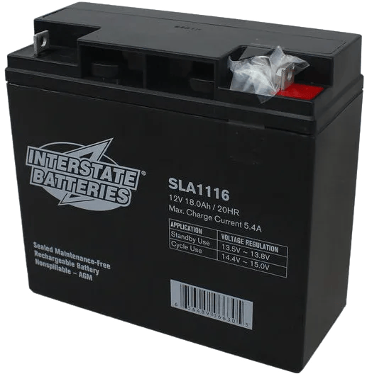
The battery is the only power source for the robot. FRC requires a specific battery type: 18 Ah, 12V sealed lead-acid. All robot power flows from this battery through the main breaker and into the PDH.
Our batteries use SB50 connectors for easy connection and disconnection from the robot. The negative/ground output from the SB50 connects directly to the PDH using a 6 AWG lug. The positive output connects to one end of the 120A main breaker, and the other end of the breaker connects to the positive input of the PDH.
Battery rules and best practices:
- Always use Anderson SB50 connectors on the battery leads. Other connectors are not legal.
- Charge batteries using an approved FRC charger only. Standard automotive chargers can damage FRC batteries.
- Label batteries with a marker so you know which are charged and which are discharged.
- Never leave a battery fully discharged for an extended period — this permanently reduces capacity.
- Check battery voltage before every match. A battery below 12.0V at rest is considered low.
- Carry multiple batteries to every competition event and make sure you check their status and age. Take the good ones to competitions.
Main Breaker
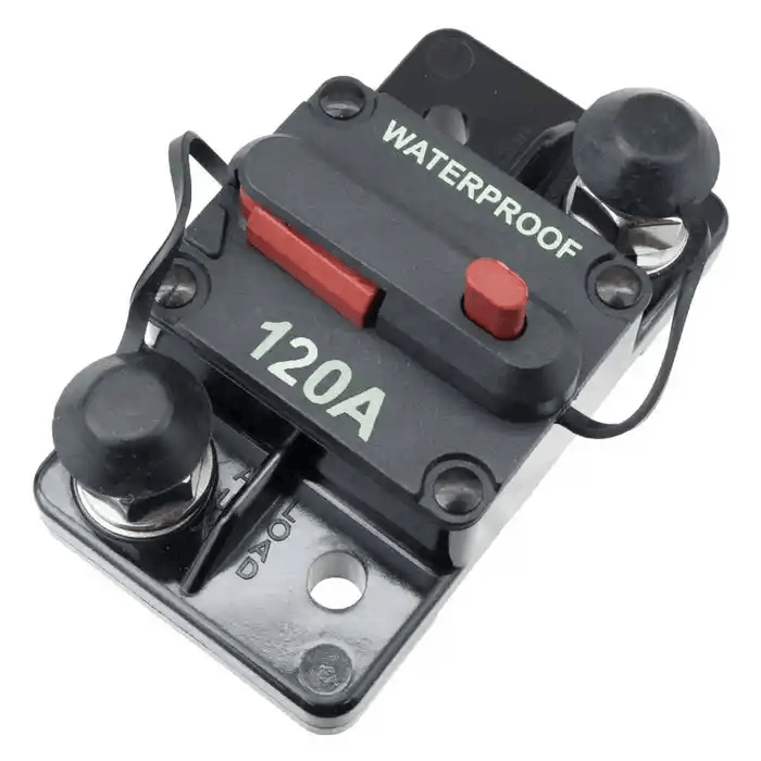
The main breaker is a 120A circuit breaker that acts as the robot’s master power switch. It sits between the battery positive terminal and the PDH positive input. Pressing the red button instantly cuts all power to the robot.
The main breaker serves two purposes: it is the primary safety disconnect (anyone can cut power quickly in an emergency), and it is the overcurrent protection for the entire robot’s power system.
Main breaker rules and best practices:
- The main breaker must be accessible from the outside of the robot frame at all times. This is an FRC inspection requirement.
- Mount it in a location that is protected from direct robot-to-robot impacts but still easy to reach.
- Wire from battery (+) → main breaker IN, then main breaker OUT → PDH (+). Battery (-) goes directly to PDH (-).
- Use 6 AWG wire with crimped lugs on both sides of the main breaker.
- Never bypass or substitute the main breaker.
Power Distribution Hub (PDH)
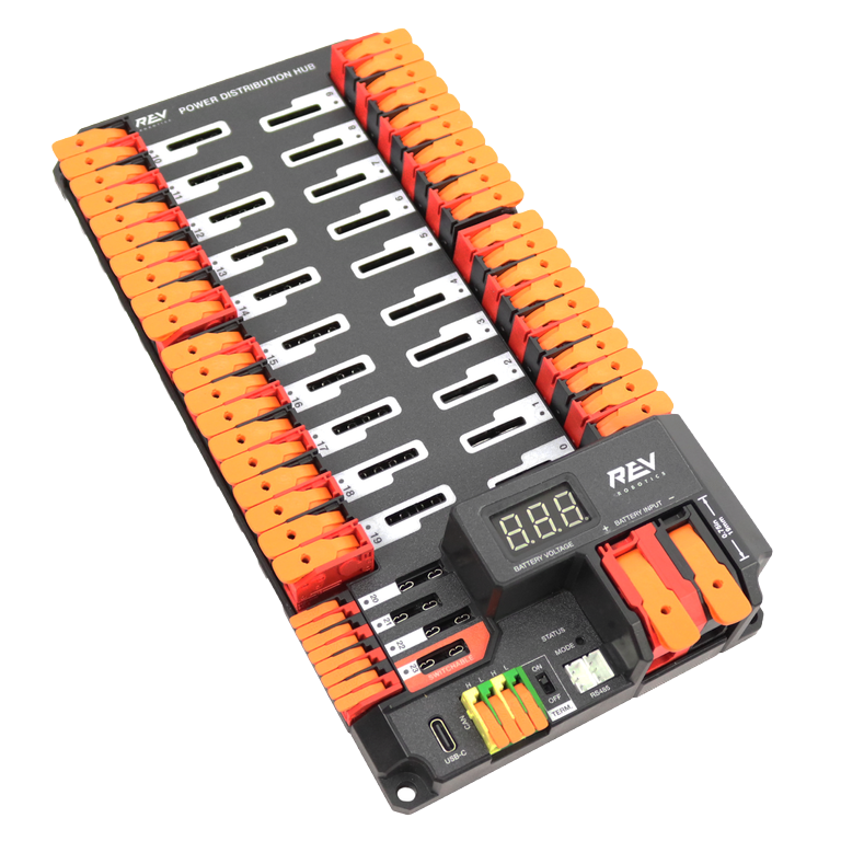
The Power Distribution Hub (PDH) is the central power distribution point for the robot. It takes power from the battery and distributes it to every motor controller, sensor, and control system component. It has 20 high-current channels (each protected by a snap-action breaker, up to 40A each) and 3 low-current channels for devices like the RoboRIO and radio.
The PDH also communicates with the RoboRIO over CAN bus, providing real-time current draw data per channel. This is useful for debugging and for monitoring robot health.
The PDH has a built-in CAN terminator, which means it must be placed at the end of the CAN chain.
Breaker sizes by component:
| Component | Breaker Size |
|---|---|
| Drive motors (Falcon 500, Kraken X60, NEO) | 40A |
| Smaller motors (NEO 550, Minion, etc.) | 20A or 30A |
| RoboRIO | 10A |
| Radio (VH-109) | 10A |
| Pneumatic Hub (PH) | 20A |
Note: Always check the FRC game manual and component documentation for the required breaker size. Using the wrong size can trip breakers during matches or damage components.
PDH best practices:
- Mount the PDH in a central, accessible location so breakers can be checked and reset quickly.
- Each channel can be switched on or off in software, which is useful for power management.
- Do not use the VRM (Voltage Regulator Module) for radio power. Power the VH-109 radio directly from a PDH 10A channel.
RoboRIO & System Core
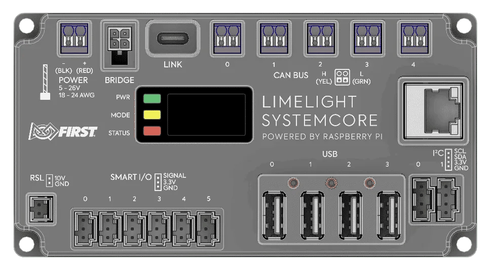
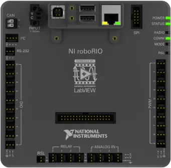
The RoboRIO (and its successor, the SystemCore) is the main controller of the robot. It runs your team’s Java/Python/C++ robot code and communicates with all other components via CAN, PWM, DIO, and ethernet.
- RoboRIO 1 and RoboRIO 2 are both legal. The RoboRIO 2 is preferred due to better performance and more onboard storage.
- The SystemCore is being introduced for the 2027 FRC season as the next-generation controller, replacing the RoboRIO.
- Both the RoboRIO and SystemCore act as CAN bus masters and are one of the two required endpoints of the CAN chain.
Wiring the RoboRIO:
- Power from a dedicated 10A breaker channel on the PDH, using 18 AWG wire.
- Connect to the PDH power input terminals using the Weidmuller push-in connectors.
- Connect to the radio via ethernet using the port labeled “RIO” on the VH-109.
- PWM headers on the RoboRIO can control motor controllers that do not use CAN.
- The RoboRIO has DIO, AIO, relay, and SPI/I2C ports for sensors and accessories.
Radio (VH-109)
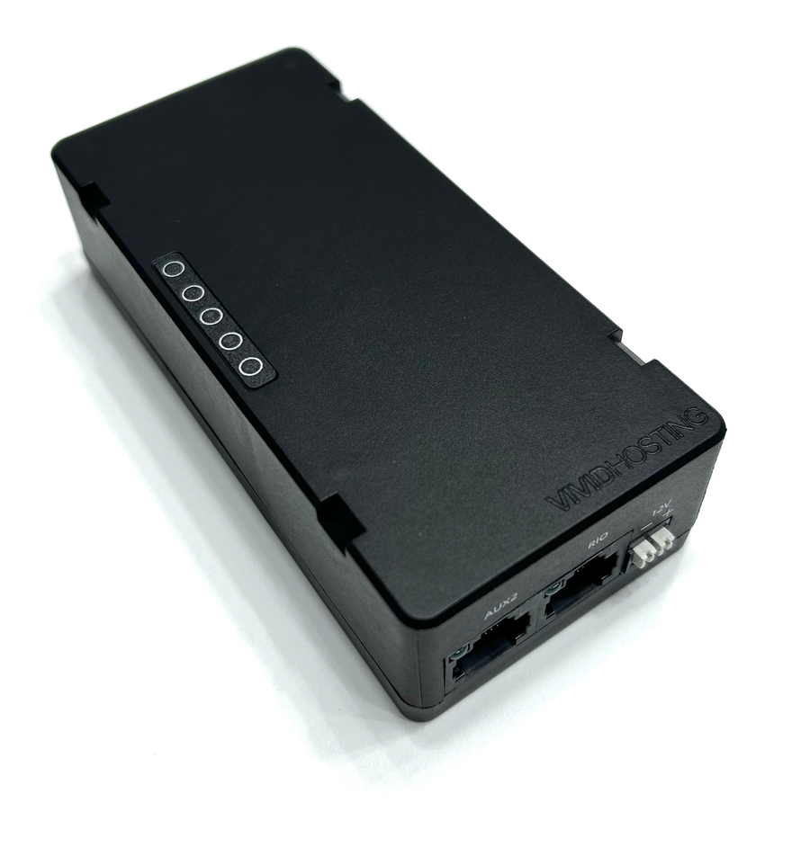
The radio for FRC is the Vivid-Hosting VH-109. It handles Wi-Fi 6E (6 GHz) communication between the robot and the Driver Station laptop. The radio must be configured at a FIRST event using the Radio Kiosk before the robot can connect to the field.
Wiring the radio:
- Power from a dedicated 10A breaker channel on the PDH, wired to the Weidmuller DC input on the VH-109.
- Connect the RoboRIO to the port labeled “RIO” on the VH-109 using an ethernet cable. Do not use any other port for this connection.
- Mount the radio so its indicator lights are visible. This lets you quickly check connection status from the pit.
Radio rules:
- The radio must be updated to the latest firmware before use at official events.
- At home practice, you need a second VH-109 acting as an access point to connect the Driver Station laptop to the robot radio. The access point radio must be powered from a wall adapter, not a battery.
- This connection can also be replaced by connecting to the radio’s wifi signal as that has the same effect. Usually 8726 doesn’t use a second radio for at home practice but that is an option.
- Do not enclose the radio in metal, as it will block the Wi-Fi signal.
Motor Controllers
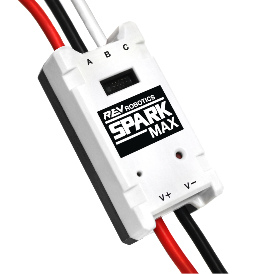
Motor controllers sit between the PDH and the motors. They receive a power input from the PDH and control how much power goes to the motor based on commands from the RoboRIO.
Common motor controllers used in FRC:
| Controller | Communication | Common Motors |
|---|---|---|
| Talon FX (inside Falcon 500 / Kraken X60) | CAN | Falcon 500, Kraken X60 (integrated) |
| Talon FXS | CAN | Minion, other brushless/brushed motors |
| SPARK MAX | CAN or PWM | NEO, NEO 550 |
| SPARK Flex | CAN or PWM | NEO Vortex |
| Thrifty Nova | CAN or USB | NEO, other brushless motors |
| Talon SRX | CAN or PWM | CIM, Mini-CIM, brushed motors |
| Victor SPX | CAN or PWM | Brushed motors (legacy use) |
Wiring a motor controller:
- Connect the controller power input (red/black) to a PDH channel with the correct breaker.
- Connect the motor output wires to the motor.
- If using CAN, daisy-chain the CAN wires through the controller.
- If using PWM, connect a PWM cable from the controller to a PWM header on the RoboRIO.
Important: Each motor controller must have a unique CAN ID set using a configuration tool (REV Hardware Client for SPARK MAX/Flex, Phoenix Tuner X for CTRE devices). Duplicate IDs will cause unpredictable behavior. See CAN Bus for details.
VRM (Voltage Regulator Module)
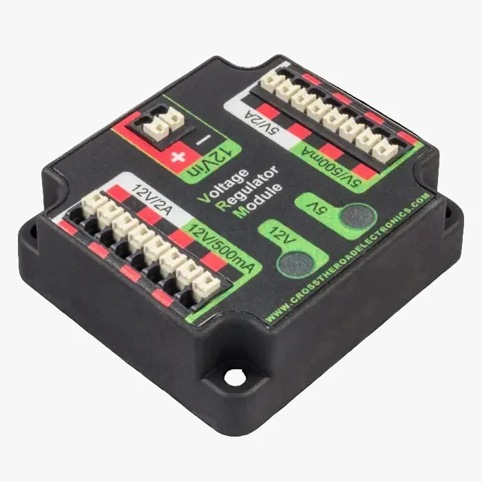
The VRM is a legacy component that provided regulated 12V and 5V outputs for cameras, sensors, and radios in older FRC setups. In current FRC configurations with the VH-109 radio, the VRM is not used for radio power.
The VRM may still be used on some robots to power custom sensors or cameras that require a regulated 12V or 5V supply, but it is not required and is not part of the standard control system wiring.
Do not use the VRM to power the VH-109 radio. The radio requires a direct PDH connection.
Safety Rules
Electrical safety is one of the most important things to get right on an FRC robot. Mistakes with wiring can damage expensive components, cause fires, or injure team members. These rules must be followed by everyone working on the robot at any time — during build season, at practice, and at competition.
Core Rules
1. Always Disconnect the Battery Before Wiring
Before touching any wire, connector, or electrical component, physically unplug the battery from the robot. It is not enough to flip the main breaker — you need to fully remove the battery connector. This ensures no current can flow through the robot while you are working on it.
Even a “dead” battery still holds enough charge to cause arcing, burns, or component damage. Always disconnect it.
2. Never Work on an Enabled Robot
Never touch any part of the robot while it is enabled in the Driver Station — not even to adjust a wire or check a connector. An enabled robot can move unexpectedly and cause serious injury. Always disable the robot and confirm it is in a safe state before approaching it.
3. Never Short Positive and Negative Wires
A short circuit occurs when the positive and negative sides of a power circuit are connected directly, bypassing any load. This causes a massive surge of current that can instantly destroy motor controllers, the PDH, the RoboRIO, or other components — and can start a fire. Always be aware of where your positive (red) and negative (black) wires are when working near exposed terminals.
4. Use the Correct Wire Gauge
Every wire on the robot has a required gauge (thickness) based on how much current flows through it. Using wire that is too thin creates resistance, which generates heat. A wire carrying more current than it is rated for will overheat, melt its insulation, and potentially start a fire. Refer to the Wire Gauges page for a full breakdown.
5. Keep Wiring Away from Moving Parts
Wires that run near gears, belts, chains, or rotating shafts can get caught and ripped out during operation. This can cause sudden loss of power to a subsystem, damage connectors, or create a short circuit. Always route wires away from moving mechanisms and secure them with zip ties.
Additional Safety Habits
- Label your wires at both ends. If something goes wrong, knowing which wire goes where will save a lot of debugging time and prevent accidentally disconnecting the wrong thing.
- Inspect wiring before every match. Vibration from matches can loosen connectors and zip ties over time. Do a quick visual check before every test run or competition match.
- Do not leave tools on the robot. Screwdrivers, wire cutters, or other metal tools left on or near the robot can fall and cause a short.
- Use insulated tools when possible. When working near powered systems (such as when checking connections on a powered-off robot that may still have capacitor charge in motor controllers), insulated tools add an extra layer of protection.
- Only one person wires at a time. Having multiple people reaching into the electrical bay at once increases the chance of mistakes. One person works, others observe and assist.
At Competition
At FIRST events, robots are inspected by referees before being allowed on the field. Electrical violations — such as exposed conductors, missing wire labels, or incorrect breaker sizes — can result in a failed inspection. Beyond inspection, unsafe wiring can cause a robot to break down mid-match or be disabled by the field system.
These rules apply at all times: during build, testing, and competition. Safety is always the top priority.
Wire Gauges
Using the correct wire gauge is one of the most important parts of safe robot wiring. Every wire on the robot carries a different amount of current depending on what it powers, and the wire must be thick enough to handle that current without overheating.
AWG (American Wire Gauge) is the standard used for wire sizing in FRC. A smaller AWG number means a thicker wire that can carry more current. For example, 6 AWG is much thicker than 18 AWG.
Quick Reference Table
| Application | Wire Gauge | Notes |
|---|---|---|
| Battery to main breaker | 6 AWG | Must use lugs, not bare wire ends |
| Main breaker to PDH | 6 AWG | Must use lugs, not bare wire ends |
| Drive motor controllers (Falcon 500, Kraken, NEO) | 12 AWG | 40A breaker circuit |
| Smaller motor controllers (NEO 550, Minion) | 18 AWG | 20A or 30A breaker circuit |
| CAN bus wiring | 22 AWG (twisted pair) | Yellow = CAN High, Green = CAN Low |
| PWM signals | Pre-made cable (provided) | Do not substitute with random wire |
| Sensor wiring (encoders, limit switches) | 22-24 AWG | Low current, signal only |
| Radio power input | 18 AWG | 10A breaker circuit |
| RoboRIO power input | 18 AWG | 10A breaker circuit |
Why Wire Gauge Matters
Every wire has a maximum current rating. If you push more current through a wire than it is rated for, the resistance of the wire causes it to heat up. At high enough temperatures the insulation melts, which can expose live conductors and cause a short circuit or fire.
This is why you should never substitute a thinner wire just because it is easier to route or already cut to the right length. If the required gauge is 12 AWG, use 12 AWG.
High-Current Runs (6 AWG)
The battery-to-breaker and breaker-to-PDH connections are the highest current runs on the robot. Under peak load, the robot can draw well over 100A through these cables. 6 AWG wire is required for these runs, and the ends must be terminated with crimp lugs — not stripped and inserted bare into a terminal.
- Use a proper hydraulic or ratchet crimper for 6 AWG lugs. Hand crimpers will not create a reliable connection at this gauge.
- Inspect these connections regularly. A loose lug on a high-current run creates significant resistance, which causes heat buildup at the connection point.
Motor Controller Wiring (12-18 AWG)
Motor controllers connect to the PDH on the input side and to the motor on the output side. The wire gauge depends on the breaker size protecting the circuit:
- 40A channels (drive motors): Use 12 AWG. This handles Falcons, Krakens, and NEOs at full load.
- 20A or 30A channels (auxiliary motors): Use 18 AWG. This is appropriate for smaller motors like the NEO 550 or Minion.
When in doubt, check the motor controller’s documentation for its recommended wire gauge on both the power input and motor output sides.
CAN and Signal Wiring (22-24 AWG)
CAN bus wires carry only small communication signals, not power, so they can be thin. However, they must be twisted together (yellow and green as a pair) to reduce electromagnetic interference from nearby high-current wires.
Sensor wiring (encoders, limit switches, beam breaks) is also low-current and uses 22-24 AWG. These wires should be kept away from motor and power wiring where possible to prevent signal noise.
Tips for Cutting and Stripping Wire
- Always use a proper wire stripper sized for the gauge you are working with. Using the wrong slot can nick the wire strands, weakening the connection.
- Strip only as much insulation as needed for the connector — leaving exposed conductor outside a terminal creates a short circuit risk.
- After crimping or inserting into a terminal, give the wire a firm tug to confirm it is secure.
Always check the FRC game manual and component documentation for required wire gauges. Requirements can change between seasons, and using the wrong gauge can result in a failed inspection or a damaged robot.
Wiring Best Practices
Good wiring is the difference between a robot that is reliable all season and one that fails mid-match due to a loose connector or a wire caught in a mechanism. This page covers the habits and techniques that keep wiring clean, secure, and easy to debug.
Cable Management
Poor cable management is one of the most common causes of robot problems. Loose wires can get snagged in mechanisms, connectors can vibrate out, and a messy wiring bay makes it very hard to trace a problem under pressure at a competition.
Routing Wires
- Plan wire routes before cutting wire to length. Route wires along the frame rails and avoid cutting across open space where possible.
- Leave a small amount of slack in every run — about 2-3 inches at each end. Wires under tension will eventually pull free from their connectors, especially after repeated matches.
- Do not route wires through areas that move, flex, or are near rotating mechanisms. Use fixed frame members as guides.
- Keep power wires (high current) and signal wires (CAN, PWM, sensors) separated where possible. Running them together for long distances can introduce electrical noise into sensor readings.
Securing Wires
- Use zip ties to bundle wires together and anchor them to the frame at regular intervals — roughly every 6-8 inches on longer runs.
- Do not over-tighten zip ties. They should hold the wire firmly without compressing the insulation. A zip tie that cuts into the insulation can damage the wire conductor over time.
- Trim the tails of zip ties flush with a diagonal cutter after tightening. Long tails are sharp and can scratch wires or people.
- Use zip tie anchor mounts (adhesive or screw-in) to create fixed attachment points on the frame when there is no convenient hole or bracket.
Wire Labels
Label every wire at both ends. When you are debugging a problem at 11 PM at a competition, you do not want to spend 20 minutes tracing a wire to figure out what it is.
- Use label tape or pre-printed labels. Color-coded electrical tape is also helpful for identifying wire pairs quickly.
- A good labeling convention is to include the component name and the pin or channel number. For example:
LEFT_DRIVE_MC_PWR+orCAN_CHAIN_3.
Connector Types
Different connectors are used for different purposes on an FRC robot. Using the right connector for each application ensures a secure, reliable connection.
| Connector | Used For | Notes |
|---|---|---|
| Anderson SB50 | Battery leads | Requires a special crimping tool. Inspect the contact for full seating. |
| Wago lever nuts | PDH main power input terminals | Flip the orange lever open, insert wire, flip closed. |
| Weidmuller push-in | PDH channel outputs, radio power | Push the wire in firmly until it clicks. Tug to confirm it is secure. |
| JST-SH / JST-GH | Sensors, encoders, small signal connectors | Commonly used on REV and CTRE sensor ports. Be gentle — these are fragile. |
| RJ45 (ethernet) | Radio to RoboRIO connection | Use a quality cable. Avoid sharp bends near the plug. |
| Phoenix Contact (screw terminal) | Some older motor controllers | Tighten screw firmly but do not overtighten — can strip the terminal. |
Keeping Connectors Secure
Vibration during a match is surprisingly aggressive. Connectors that seem solid on the bench can work loose after a few matches.
- Use small zip ties around connector pairs to prevent them from separating under vibration.
- For critical connections like motor controller power leads, consider using electrical tape or cable clamps in addition to zip ties.
- Always do a tug test on every connector after you make it. If it comes out with light force, re-seat it or investigate whether the terminal is properly crimped.
Protecting Wires
Split Loom and Cable Sleeves
When wires must pass through an area with rough edges, moving parts, or tight quarters, protect them with split loom tubing or braided cable sleeve. This prevents abrasion that can wear through insulation over time.
- Size split loom to the bundle — too small and you cannot fit all the wires in, too large and it flops around and may not stay in place.
- Secure the ends of split loom with a zip tie or electrical tape to prevent it from sliding.
Grommets
Any time a wire passes through a hole in sheet metal or a frame extrusion, use a rubber grommet in the hole. Sheet metal edges are sharp enough to cut through wire insulation over time, especially with vibration. Grommets create a smooth, rounded surface for the wire to contact.
Heat Exposure
- Avoid routing wires near motors or motor controllers, as they generate significant heat during operation. Sustained heat exposure degrades insulation.
- If you must route wires near a heat source, use high-temperature wire or add additional insulation like fiberglass sleeve.
Electrical Tape and Heat Shrink
- Electrical tape is useful for bundling wires, covering exposed connectors, and adding a secondary layer of insulation. Do not rely on it as a substitute for proper insulation — it can unravel over time, especially in warm environments.
- Heat shrink tubing is the preferred way to insulate exposed solder joints or crimped connections. It creates a permanent, durable seal. Always use the correct diameter and apply heat evenly with a heat gun. Avoid using an open flame.
General Habits
- Cut wires to length. Do not coil up excess wire and zip tie the bundle. Extra wire adds weight and creates a tangled mess that is hard to service. Measure, cut, and route precisely.
- Use the right tool for each job. Strip wire with a proper wire stripper. Crimp with a proper crimper. A sharp knife and pliers are not substitutes — they lead to damaged wires and poor connections.
- Document your wiring. Keep a wiring diagram or spreadsheet that lists every PDH channel, what is connected to it, the breaker size, and the CAN ID if applicable. This is invaluable during troubleshooting.
Robot Wiring Order
When wiring a new robot (or rewiring after major mechanical changes), following a consistent order keeps the process organized and reduces the chance of mistakes. This order ensures that each step builds on the last — you are never connecting something before what it depends on is already in place.
Before you start: Make sure the battery is disconnected and no one is powering the robot during the wiring process.
Step 1 — Mount the Core Electrical Components
Before running any wire, mount all of the main electrical components to the robot frame in their final positions. This lets you plan wire routes accurately and cut wires to the correct length.
Components to mount:
- PDH (Power Distribution Hub) — Central location on the frame, accessible from the outside.
- RoboRIO — Secure location, protected from direct hits, accessible for USB connection during programming.
- Main breaker — Must be accessible from the outside of the robot frame per FRC rules.
- Radio (VH-109) — Elevated location where its indicator lights are visible. Avoid metal enclosures that block Wi-Fi signal.
- Motor controllers — Mounted near the motors they control to keep motor output wires short.
Step 2 — Run the Main Power Cables
This is the backbone of the robot’s electrical system. These are the highest-current wires on the robot and must be done first.
- Connect the battery to the main breaker IN terminal using 6 AWG wire with crimped lugs.
- Connect the main breaker OUT terminal to the PDH positive input using 6 AWG wire with crimped lugs.
- Connect the battery negative directly to the PDH negative input using 6 AWG wire with crimped lugs.
Do not connect the battery yet. Route and secure these cables, but leave the battery disconnected until all wiring is complete and inspected.
Step 3 — Wire RoboRIO Power
The RoboRIO must have a dedicated 10A breaker channel on the PDH.
- Select a 10A breaker channel on the PDH and insert a 10A snap-action breaker.
- Run 18 AWG wire from that PDH channel to the RoboRIO power input terminals (marked + and -).
- Connect the wires to the RoboRIO’s Weidmuller power input. Red (+) to the positive terminal, black (-) to the negative terminal.
- Tug both wires to confirm they are fully seated.
Step 4 — Wire Radio Power
The VH-109 radio is powered directly from a PDH channel, not through a VRM. This is an important distinction from older FRC radio setups.
- Select a 10A breaker channel on the PDH and insert a 10A breaker.
- Run 18 AWG wire from that PDH channel to the Weidmuller DC input on the VH-109.
- Do not use the VRM (Voltage Regulator Module) to power the radio. The VH-109 requires a direct PDH connection.
Step 5 — Connect RoboRIO to Radio
- Run a quality ethernet cable from the RoboRIO ethernet port to the port labeled “RIO” on the VH-109.
- Use the correct port — plugging into the wrong port on the radio can prevent communication or damage the radio.
- Secure the ethernet cable with zip ties so it cannot be pulled loose during a match.
Step 6 — Wire Motor Controllers
For each motor controller on the robot:
- Select a PDH breaker channel appropriate for the motor (40A for drive motors, 20-30A for smaller motors).
- Insert the correct snap-action breaker for that channel.
- Run the appropriate gauge power wire (12 AWG for 40A channels, 18 AWG for smaller channels) from the PDH channel to the motor controller power input.
- Connect the motor output wires from the controller to the motor terminals.
- If the motor controller uses CAN, leave the CAN connections for Step 7.
- If the motor controller uses PWM, connect a PWM cable from the controller signal input to the appropriate PWM header on the RoboRIO.
Repeat this for every motor controller on the robot before moving on.
Step 7 — Run the CAN Bus Chain
CAN devices must be wired in a daisy chain from the RoboRIO to the PDH. The PDH must be at the end of the chain because it has the built-in terminator.
- Start at the RoboRIO CAN port (yellow = CANH, green = CANL).
- Run CAN wire to the first device in the chain, connecting CANH to CANH and CANL to CANL.
- Continue daisy-chaining through each CAN device (motor controllers, Pneumatic Hub, etc.).
- End the chain at the PDH CAN port. The PDH’s built-in terminator closes the bus.
- Twist yellow and green wires together for any run longer than about 6 inches to reduce interference.
After completing the chain, use REV Hardware Client and Phoenix Tuner X to assign unique CAN IDs to every device before powering the full system. See CAN Bus for details.
Step 8 — Connect Signal Cables (PWM, Sensors, Encoders)
With the power and CAN wiring done, connect all remaining signal cables.
- PWM cables: Connect from motor controllers to the RoboRIO PWM headers. Match the signal pin to the correct header number as defined in your code.
- Encoders and sensors: Connect sensor signal cables to the appropriate DIO, AIO, or sensor ports on the RoboRIO.
- Limit switches and beam breaks: Wire to the DIO ports on the RoboRIO.
- Route all signal cables away from high-current power wires to reduce noise.
Step 9 — Label Every Wire and Secure Cable Runs
Before doing a final inspection, label every wire at both ends and secure all cable runs with zip ties.
- Labels should identify the component and connection point (e.g.,
LEFT_FRONT_DRIVE_+orCAN_CHAIN_2). - Use zip tie anchor mounts to secure wire bundles to the frame at regular intervals.
- Trim all zip tie tails flush.
- Check that no wires cross near gears, belts, or other moving mechanisms.
Step 10 — Visual Inspection Before Connecting the Battery
Before connecting the battery, do a thorough visual inspection:
- Check every power connection for correct polarity (red = +, black = -).
- Check that all PDH breakers are installed and seated properly.
- Confirm all CAN connections are secure and the chain runs from the RoboRIO to the PDH.
- Confirm no bare wire conductors are exposed outside of connectors.
- Confirm no wires are near moving mechanisms.
- Verify that the main breaker is in the OFF (popped/reset) position before connecting the battery.
Once the inspection passes, connect the battery and power on the robot to test communication.
CAN Bus
CAN (Controller Area Network) bus is the primary communication network on an FRC robot. It connects the RoboRIO to smart devices like motor controllers, the PDH, and the Pneumatic Hub using just two wires. Understanding how CAN works — and how to set it up correctly — is essential to getting a robot that runs reliably.
What is CAN Bus?
CAN bus is a two-wire serial communication protocol originally developed for automotive use. On an FRC robot, it allows the RoboRIO to send commands to and receive data from smart devices at high speed.
The two wires are:
- CAN High (CANH) — Yellow wire
- CAN Low (CANL) — Green wire
Data is transmitted as a differential signal between these two wires. Because the signal is differential (not referenced to ground), CAN bus is naturally resistant to electrical noise — which is why it works well near the high-current wiring found on FRC robots.
How CAN Bus is Wired
CAN devices must be wired in a daisy chain topology — each device connects to the next in a single continuous line. The two endpoints of the chain must be terminated. On an FRC robot:
- The RoboRIO is always one endpoint (it is the CAN bus master)
- The PDH is always the other endpoint (it has a built-in 120Ω termination resistor)
Note
With the release of System Core for the 2027 FRC Season we will most likely be starting multiple parrallel CAN bus chains at the SystemCore. For this reason, we will also need seperate 120Ω resisters to terminate the CAN. Also, the CAN bus does NOT HAVE to terminate at the PDH. We usually keep it this way to avoid having another resister but it can be terminated anywhere with a resister.
RoboRIO --> Device 1 --> Device 2 --> Device 3 --> ... --> PDH (termination)
The order of devices in the middle of the chain does not affect function. What matters is that the RoboRIO and PDH are at the two ends.
Wiring rules:
- Connect CANH to CANH and CANL to CANL throughout the chain. Do not cross the wires.
- Twist the yellow and green wires together for any run longer than about 6 inches. Twisting reduces electromagnetic interference (EMI) from nearby high-current motor wiring.
- Keep CAN wires as far from high-current power cables as is practical.
- Do not use a star (branching) topology. CAN bus must be a single continuous chain with no branches.
- Use 22 AWG twisted pair wire for all CAN runs.
CAN IDs
Every device on the CAN bus must have a unique ID number. IDs are assigned by the user using configuration software before the device is added to the bus. Most motor controllers ship with a default ID of 0 or 1, which means if you add multiple controllers to the bus without configuring them first, they will all have the same ID and conflict with each other.
Why Unique IDs Matter
When two devices share the same CAN ID, they both respond to commands meant for that ID and both transmit data on it at the same time. This causes bus collisions and errors. One or both devices may stop responding, and the errors can affect all other devices on the bus as well. This is one of the most common causes of motor failures at competition.
How to Set CAN IDs
For REV devices (SPARK MAX, SPARK Flex):
- Connect the motor controller to your computer via USB.
- Open REV Hardware Client.
- Select the device from the list.
- Change the CAN ID to the desired value and click “Update”.
- Disconnect the USB before adding the device to the CAN bus.
For CTRE devices (Talon FX, Talon FXS, Talon SRX, Victor SPX):
- Connect the motor controller to your computer via USB (or connect it to the robot with CAN and USB).
- Open Phoenix Tuner X.
- Select the device from the device list.
- Set the ID field to the desired value and click “Set”.
- Confirm the ID change before proceeding.
Recommended CAN ID Conventions
Keeping CAN IDs organized by subsystem makes debugging much easier. Here is one common convention:
| ID Range | Use |
|---|---|
| 0-5 | Gyro, PDH, Rio, etc |
| 10-12, 20-22, 30-32, 40-42 | Drive encoders, steering motors, and drive motors |
| 50+ | Mechanisms - Usually grouped together |
| 60+ | Sensors and other Misc (Also can go in 1-10) |
The actual convention your team uses does not matter as long as it is consistent and documented.
Keeping a CAN ID Record
Always maintain a written or digital record of every CAN ID assignment. A simple spreadsheet works well:
| CAN ID | Device Type | Mechanism | Notes |
|---|---|---|---|
| 1 | Talon FX | Left Front Drive | Inverted in code |
| 2 | Talon FX | Left Rear Drive | Inverted in code |
| 3 | Talon FX | Right Front Drive | |
| 4 | Talon FX | Right Rear Drive | |
| 10 | SPARK MAX | Arm | NEO motor |
| 11 | SPARK MAX | Wrist | NEO 550 |
| 20 | SPARK Flex | Intake | NEO Vortex |
This record should be version-controlled alongside your robot code.
Note
8726 uses a PDH Diagram which can be found here.(Might require access to team drive but it can be found online somewhere) This serves as a good holder for the wiring charts/diagrams and CAN ids.
Checking CAN Bus Health
The CAN bus status can be monitored in real time from the Driver Station.
- Open the Driver Station and click the lightning bolt icon or go to the Diagnostics tab.
- The CAN Bus Utilization percentage should stay below 90% during normal operation. High utilization can cause delays and missed messages.
- CAN Bus errors should be zero at all times. Any non-zero error count indicates a problem that needs to be investigated.
Common CAN Bus Problems and Fixes
| Symptom | Likely Cause | Fix |
|---|---|---|
| CAN errors in the DS | Loose or broken CAN wire | Inspect the entire CAN chain for loose connections |
| CAN errors in the DS | Duplicate CAN IDs | Check IDs in Phoenix Tuner X and REV Hardware Client |
| One device not responding | Break in the daisy chain at that device | Check CAN wires at the problem device |
| All devices stopped responding | Missing termination (PDH disconnected from chain) | Verify PDH is at the end of the chain and CAN wires are connected |
| Intermittent CAN errors | CAN wires not twisted, near power cables | Re-route and twist CAN wires away from motor wiring |
CAN vs PWM
Some motor controllers support both CAN and PWM communication. Here is a comparison:
| Feature | CAN | PWM |
|---|---|---|
| Wires required | 2 (shared bus) | 3 per controller |
| Feedback (current, temp, velocity) | Yes | No |
| Configuration options | Full | Limited |
| Fault detection | Yes | No |
| Recommended for | All new robots | Legacy setups only |
CAN is strongly preferred for all motor controllers. Use PWM only when a CAN controller is not available or as a fallback.
Pre-Match Checklist
This checklist should be run before every match and every significant test session. Electrical problems that are caught in the pits are much easier to fix than ones that show up on the field. Make this a routine — it only takes a few minutes and can prevent a lost match.
Tip: Assign one person on the drive team or pit crew to own this checklist. It should be completed by the same person every time so nothing gets missed.
Battery
- Battery is fully charged (check voltage with a voltmeter or the DS — should be 12.5V or above at rest)
- Battery connector (Anderson SB50) is fully seated and locked into the robot
- Battery is physically secured in its mount and cannot shift during a match
- No other batteries are sitting loose in the robot
Main Breaker
- Main breaker is accessible from the outside of the robot frame
- Main breaker is in the ON (reset) position — button is not popped out
- Main breaker wiring (6 AWG lugs) is tight and not pulling away from the terminals
Power Distribution Hub (PDH)
- All snap-action breakers are fully seated in their channels (press each one down firmly)
- No breakers are tripped (check the LED indicators on the PDH if visible)
- PDH mounting bolts are tight — a loose PDH can cause intermittent power issues
- PDH to RoboRIO and PDH to radio power wires are secure (tug test)
Wiring and Connectors
- No loose wires or connectors visible anywhere on the robot
- No wires are crossing near gears, belts, chains, or rotating shafts
- No wire bundles are pulled tight or under tension
- All motor controller power connectors are secure (tug each one)
- All motor output connections are secure
- Ethernet cable between RoboRIO and radio is firmly seated at both ends
CAN Bus
- Driver Station shows 0 CAN Bus errors (check the DS diagnostics tab)
- CAN utilization shown in the DS is below 90%
- All expected CAN devices are visible and responding (verify in REV Hardware Client or Phoenix Tuner X if there is time)
Radio
- Radio indicator lights show the correct status for field connection (solid green or blue depending on the event)
- Radio is physically secured and not at risk of being knocked loose
- Ethernet cable is connected to the correct “RIO” port on the VH-109
Driver Station
- Driver Station shows green communication with the robot
- No robot code errors or warnings in the DS log
- Robot mode is set to Teleop (or the correct mode for the situation) before enabling
- Joysticks and controllers are recognized and responding correctly in the DS
- Battery voltage reading in the DS is reasonable (12.0V or above when idle)
Final Physical Check
- All access panels, bumper brackets, and covers that were moved during pit work are properly secured
- No tools, loose hardware, or foreign objects are sitting inside the robot
- Robot is in its starting configuration for the match
After a Match — Quick Damage Check
Run this quick check after every match before the robot goes back to the pit:
- No smoke, burning smell, or visible scorch marks anywhere on the robot
- No wires visibly pulled out or dangling
- No breakers tripped on the PDH
- Main breaker is still in the ON position
- Battery connector is still fully seated
If any of these fail, do not run the robot again until the issue is found and resolved.
Common Mistakes
Every electrical team makes mistakes, especially early in build season. This page documents the most common wiring errors seen in FRC robots, explains why they happen, and tells you how to avoid or fix them.
Reversed Polarity
What it is: Connecting the positive (+) wire to a negative terminal, or the negative (-) wire to a positive terminal.
Why it happens: Wires are cut and labeled incorrectly, or color conventions are not followed consistently. It is most common on motor output wires where both leads look similar.
What happens: Reversed polarity on motor controllers can destroy them instantly. Some controllers have protection against this, but many do not. On motors, reversed polarity causes the motor to spin backwards — which may not be immediately obvious and can cause mechanical damage if a mechanism is driven in the wrong direction.
How to avoid it:
- Always use red for positive and black for negative on power wires. Do not improvise.
- Double-check polarity before connecting any power cable.
- Use a multimeter to verify polarity at both ends of a run before connecting.
- Label both ends of every wire as part of the wiring process, not as an afterthought.
Wrong Breaker Size
What it is: Installing a breaker that is too large or too small for the circuit it is protecting.
Why it happens: Teams grab whatever breaker is available without checking the spec, or assume that a larger breaker is “safer” because it is less likely to trip.
What happens: A breaker that is too large will not trip when it should, meaning the wire it protects can overheat and potentially start a fire before the breaker responds. A breaker that is too small will trip repeatedly during normal operation, causing unexpected robot shutdowns during matches.
How to avoid it:
- Refer to the Wire Gauges page and the FRC game manual for correct breaker sizes.
- Do not substitute breaker sizes based on what you have in stock. Order the correct size.
- Label each PDH channel with the breaker size and what it powers.
Duplicate CAN IDs
What it is: Two or more devices on the CAN bus assigned the same ID number.
Why it happens: Motor controllers from the factory often default to ID 0 or ID 1. If you add multiple controllers to the bus without configuring them individually, they will all have the same ID.
What happens: Devices with duplicate IDs will conflict on the bus. One or both devices may stop responding, behave erratically, or cause CAN bus errors that affect all other devices on the bus. This is one of the most common causes of mysterious motor failures at competition.
How to avoid it:
- Set CAN IDs before connecting a new device to the CAN bus. Configure it alone first.
- Use REV Hardware Client for SPARK MAX and SPARK Flex.
- Use Phoenix Tuner X for CTRE devices (Talon FX, Talon FXS, Talon SRX, Victor SPX).
- Keep a written record (spreadsheet or wiring diagram) of every CAN ID and what device it belongs to.
- Check the CAN bus status in the Driver Station before every match. Zero errors is the goal.
Unsecured Connectors
What it is: Connectors that are not physically anchored and can vibrate or pull loose.
Why it happens: During wiring, connectors are seated and tested on a stationary bench. Vibration from a match is very different from static conditions. A connector that feels solid on the bench can work loose after one or two matches.
What happens: An unsecured connector can pull free during a match, cutting power or communication to a motor or the RoboRIO. This often looks like a random failure with no obvious cause.
How to avoid it:
- Zip-tie connectors together or anchor them to the frame so they cannot separate.
- For Weidmuller push-in connectors, give every wire a firm tug after insertion to confirm it is locked.
- For Anderson SB50 battery connectors, inspect the spring contact inside for proper tension.
- After every match, do a quick tug test on critical connectors.
Wires Cut Too Short
What it is: Wires that are too short and are pulled tight between their endpoints.
Why it happens: Wires are measured and cut when the robot is in a specific configuration. When the robot moves or a mechanism shifts, the slack disappears and the wire is stretched tight.
What happens: A wire under constant tension will eventually fatigue and break at the connector crimp or terminal. This usually happens during or just before a match and can be very difficult to diagnose because the break may not be visible.
How to avoid it:
- Always leave 2-3 inches of slack at each end of every wire run.
- Before finalizing wire routes, move the robot through its full range of motion and verify that no wire becomes tight.
- Pay special attention to wires that cross between the robot frame and a moving mechanism (like a rotating arm or elevator).
No Wire Labels
What it is: Wires that are not labeled, making it impossible to identify them without tracing the full run.
Why it happens: Labeling feels slow and tedious, especially when the team is rushing to get the robot ready. Labels get skipped with the intention of doing them later, which often never happens.
What happens: When a problem occurs (and problems always occur), unlabeled wiring makes debugging dramatically slower. At a competition with limited time between matches, spending 20 minutes tracing a wire can cost you a match.
How to avoid it:
- Make labeling a required part of the wiring process. Do not consider a wire finished until it is labeled at both ends.
- Use a consistent naming convention so labels are immediately meaningful (e.g.,
LEFT_REAR_DRIVE_+,CAN_TO_PDH_H). - Even simple color-coded tape on bundles helps when the full label is not readable at a glance.
Wrong Radio Ethernet Port
What it is: Plugging the RoboRIO ethernet cable into the wrong port on the VH-109 radio.
Why it happens: The VH-109 has multiple ethernet ports and they are not all the same. The port for the RoboRIO is specifically labeled “RIO” and it is the only port that should be used for this connection.
What happens: Using the wrong port will prevent robot communication. In some cases it can also damage the connected device. The robot will appear to have no communication even though the radio is powered and the ethernet cable is connected.
How to avoid it:
- Always connect to the port labeled “RIO” on the VH-109.
- Mark the correct port with a small piece of colored tape after initial setup so it is always obvious which port to use.
Running Wires Near Moving Parts
What it is: Routing a wire through or near a mechanism that moves, rotates, or flexes during operation.
Why it happens: Space is tight on FRC robots, and the shortest path for a wire often crosses through an area that a mechanism also uses. During initial wiring it may not be obvious that a mechanism will reach a wire once the robot is running.
What happens: The mechanism catches the wire, either ripping it out at the connector, cutting through the insulation, or breaking the wire. This can cause a sudden loss of power or a short circuit.
How to avoid it:
- Run the robot through its full range of motion before finalizing wire routes.
- Use flexible wire (stranded, not solid core) for any run that must cross near a moving mechanism.
- When a wire must pass near a moving part, use split loom to protect it and secure it so it cannot be pulled into the mechanism.
Programming Guide
This section provides an introductory guide to various concepts involved in FRC programming and should give you all the information you need to get started writing code on this team, as well as some resources.
Most information related to robot code and programming can be found on the WPILib Official Documentation, so if you have additional questions, you should look there.
(Needs proofreading! Written by: Dhruva)
Overview of WPILib and Robot Code
Basics of Robot Code
Our team uses Java to program our robots. This code is run on the robot’s central processor, either in a roboRIO (used in previous years) or a SystemCore (used after 2026). Code run here will be able to control any devices connected to the roboRIO or SystemCore via USB, Ethernet, or CAN, and communicate with the FMS (Field Management System) or a laptop during testing to react to inputs from the driver and send/receive other data over the network such as camera streams or debugging info.
Note
There are many publicly available resources for gaining a basic understanding of Java, such as w3schools and codecademy. Basic skills with Java are obviously necessary to write robot code and all control members will learn some basic Java. However, this guide will not teach you basic Java programming skills.
Java code is written in plain text in .java files, and then compiles to a .jar file. The compiled .jar file can be run by a program called the Java Virtual Machine, so it can easily be run either by the robot or on team laptops to simulate robot code for debugging purposes. Most of these processes are automated and described in the later How do we build and deploy robot code? section.
What is WPILib?
WPILib is a library and suite of tools designed for use when programming FRC robots. As a library, it contains a lot of useful code we can access in the form of Java classes. This greatly simplifies interfacing with common things in FRC and performing common tasks such as running certain types of control theory. WPILib also provides a general project structure and several frameworks such as Commands which we make use of when programming the robot.
Additionally, WPILib comes with several other tools. These are explained in more detail in their dedicated section in the software chapter, but include tools for debugging such as Glass as well as a custom build of Visual Studio Code which we typically use for development.
We also use several other libraries in our robot code, such as REVLib and PhoenixLib which contain utilities to interact with REV and CTRE Phoenix devices. These libraries are managed through WPILib’s vendor dependency system. To view and manage vendor dependencies, click on the WPILib logo on the far left of VS Code, which will open this menu:
How do we write robot code?
Our team primarily writes robot code in WPILib’s custom build of VS Code, which also allows us to easily simulate and debug robot code, and has standard useful features such as autocomplete and error highlighting. We also use Git to track changes made to robot code and host it on GitHub so everyone on the team can have shared access to the code (for more information on these see their dedicated section).
Beyond that, most of it is a standard Java project. Please be sure to document your code where necessary to make life easy for others - remember, other people need to read your code too!
Note
This VS Code build uses Red Hat’s Java LSP support, which is… awful. It often takes a while to start up, so if you don’t see autocomplete or errors/warnings popping up after starting VS Code, you may need to wait a few seconds. However, if it takes longer than ~1 minute, you may need to run then
Java: Clean Java Language Server Workspacecommand in VS Code, and then when you clickReload and Deleteit should start working after a few seconds. This happens A LOT, especially on team laptops.
How do we build and deploy robot code?
WPILib projects are built using Gradle. Gradle is a build system which handles dependencies,
versioning, build options, and the entire compilation process. It is configured in the build.gradle file at the root
of any WPILib project, however,
most tasks you need to do are abstracted by WPILib so you likely will not need to edit this file. In order to run
gradle or specific tasks in gradle, you can run the gradlew (mac/linux) or gradlew.bat (windows) scripts, however
most things you may need to do can be run more quickly as VS Code commands added in WPILib’s build of VS Code.
Pressing Ctrl+Shift+P brings up the command prompt in VS Code, and if you search for WPILib you can see all of the
commands added by WPILib. You can also click the WPILib logo in the top right corner to quickly bring up these commands.
If you run Build Robot Code, a .jar file will be built containing the compiled robot code. If there have been any changes to
the dependencies since that last time robot code was built, this will require internet and may take some time while
new/updated dependencies are downloaded.
Running Simulate Robot Code will first build the robot code and then simulate it on your computer. It is
generally recommended to choose the Sim GUI option, which
opens Glass so you can view information about the code and send inputs to the robot.
Running Deploy Robot Code is how we actually get robot code onto the robot. This will automatically connect to
the robot via internet if you are on the radio’s WiFi or tethered to it by an ethernet cable. Then, robot
code is built, and the .jar file along with everything in the src/main/deploy/ directory is copied over to the robot’s
internal storage. The src/main/deploy directory is often used to send information generated by other programs such as
Choreo, PathPlanner, and the configuration for our robot’s swerve drive, which will be explained in later sections.
How is robot code organized?
Our robot code follows WPILib’s project structure.
Inside the src/main folder there is a java folder containing all java source
code and a deploy folder containing other files that should be copied over to the
robot. Within the java folder all our code should be contained in frc/robot.
The Main.java file contains the entry point. You should not edit this.
Robot.java contains mostly boilerplate and is rarely edited. RobotContainer.java contins
most of the larger logic around the robot, and its constructor contains tasks run on startup.
Then, we have some utility files such as util/Constants.java which contains various
constant values for physical information or settings.
The bulk of robot code is organized into separate “subsystems” which usually follow
the physical subsystems on the robot (intake, outtake, arms, elevators, shooters, etc).
These are in the subsystems folder (duh).
(Needs proofreading! Written by: Keshav)
Interfacing with Physical Devices
Robot code is only useful when it can read what is happening on the robot and make physical hardware do something. Motors, encoders, gyroscopes, switches, pneumatics, LEDs, cameras, and power-distribution devices all need a Java object that allows our code to communicate with the real device.
This page explains the patterns shared by almost every physical device in FRC. The pages on REV motors, CTRE motors, sensors, and cameras explain their specific APIs in more detail.
The Complete Path from Code to Hardware
When we write something like
motor.setVoltage(6.0);
Java is not directly changing the voltage on a wire. Several layers are involved:
- Our subsystem calls a method on a Java object.
- WPILib or a vendor library turns that call into data understood by the device.
- The roboRIO or SystemCore sends that data through CAN.
- The physical controller receives the data and changes an output.
- Sensors send measurements back through the same interface.
- Our code reads those measurements during a later robot loop.
The Java object is our software representation of the physical device. Constructing it does not construct new hardware, obviously. It tells the library what device exists and how to reach it.
Because every layer must agree, a problem that looks like a code problem may actually be:
- An incorrect CAN ID or port number
- A missing vendor library
- An unplugged or incorrectly wired device
- A device with old firmware
- A sensor reporting different units than expected
- Two devices configured with the CAN ID
- A configuration that never reached the device
Understanding the entire path makes these problems much easier to diagnose.
WPILib and Vendor Libraries
What WPILib Provides
WPILib contains Java classes for hardware connected directly to standard robot-controller ports and for several common FRC devices. Some examples include:
PWMMotorControllerimplementations for PWM motor controllersMathUnits- and many many more
These classes are included in a normal WPILib Java project. Their packages usually begin with:
edu.wpi.first.wpilibj
Command-based classes use:
edu.wpi.first.wpilibj2.command
Math and controller classes generally use:
edu.wpi.first.math
Imports matter because two libraries may have classes with similar names. Let VS Code autocomplete the class and inspect the import it adds instead of guessing.
Why Vendor Libraries Exist
WPILib cannot contain the complete API for every piece of hardware made by every FRC vendor. Manufacturers publish their own Java libraries for devices that have features beyond the standard WPILib interfaces.
Our most common examples are:
- REVLib for SPARK motor controllers and other REV devices
- Phoenix 6 for CTRE Talon FX, CANcoder, Pigeon, and other CTRE devices
- YAGSL for swerve control
- PathPlanner and Choreo for autos
A vendor library contains:
- Java classes used by our code
- Code for communicating with the device
- Configuration objects and status/error types
- Native libraries needed on the robot
- Sometimes simulation support
The hardware may be wired and visible on the CAN bus while our code still cannot use it until the correct vendor dependency is installed.
Installing a Vendor Dependency
Vendor dependencies are managed per project. Installing REVLib in one robot project does not automatically add it to another project.
In current WPILib VS Code:
- Click the WPILib icon in the Activity Bar to open the Dependency Manager.
- Find the required library.
- Select Install.
- Allow the project to rebuild.
Libraries can also be installed from a vendor JSON URL or from an offline vendor installation. The dependency description is copied into the project’s vendordeps/ folder. That JSON file tells Gradle which Java, native, and simulation libraries the project needs.
Commit files in vendordeps/ to Git. Everyone building the project and the robot deployment must use compatible dependency versions.
Important
Do not copy a random vendor JSON from a different season without checking compatibility. WPILib and vendor libraries release year-specific versions, and an old library may not work with the current robot project or firmware.
Updating Vendor Libraries
Updating a library changes code used by the entire robot, so treat it like a real code change:
- Read the vendor’s release notes and migration guide.
- Update through the WPILib Dependency Manager.
- Build the project.
- Fix changed or removed APIs.
- Verify device firmware compatibility.
- Test in simulation when supported.
- Test every affected mechanism on the real robot.
Avoid unnecessary dependency updates immediately before an event. Once a robot is working reliably, known versions are usually more valuable than a new feature we do not need.
Finding API Documentation
There are three particularly useful sources when working with a device:
- The vendor’s programming guide explains intended workflows and important warnings.
- Java API documentation, or Javadocs, lists classes, constructors, and methods.
- Example projects show how the parts fit together in real robot code.
Use WPILib: Open API Documentation from the Command Palette for WPILib Javadocs. Vendor documentation is linked from the REV and CTRE Phoenix sites.
Autocomplete shows what methods exist, but it does not replace reading the documentation. A method accepting a double does not tell us whether that number represents rotations, radians, meters, percent output, volts, or something else.
Types of Physical Devices
Actuators
An actuator changes the physical world.
Common FRC actuators include:
- Motors
- Pneumatics
- Servos
- Relays and switched power channels
- LEDs
Actuators receive outputs from robot code. Many smart actuators also return measurements, faults, temperature, current, or configuration information.
Sensors
A sensor measures the robot or its environment.
Common examples include:
- Relative and absolute encoders
- Gyroscopes
- Limit switches and beam-break sensors
- Cameras and vision coprocessors
Sensors may be connected directly to the robot controller or built into another device. A SPARK or Talon FX, for example, can both control a motor and report encoder measurements.
Infrastructure and Diagnostic Devices
Power distribution and pneumatic controllers are not mechanism actuators in the same way a motor is, but their data is extremely valuable:
- Battery voltage
- Per-channel current
- Total current
- Temperature
Reading these values can explain brownouts, stalled motors, disconnected mechanisms, and other problems that position alone cannot reveal.
How Devices Connect
| Interface | Common devices | How devices are identified | Important characteristics |
|---|---|---|---|
| CAN | Smart motor controllers, CANcoders, Pigeons, PDH, Pneumatic Hub | CAN ID and sometimes CAN bus name | Two-way communication, configuration, telemetry, and faults |
| USB | Cameras, serial sensors, and coprocessors | USB device or serial port | General-purpose connection; enumeration can matter |
| Ethernet | Cameras, coprocessors, radio, robot controller | IP address, hostname, or network service | High-bandwidth network communication |
The electrical connection determines which Java class and constructor we use. A limit switch connected to DIO uses a different API from a CAN-based sensor even if both ultimately tell us whether something has reached a limit.
CAN IDs
Every device on the same CAN bus must have an appropriate, unique CAN ID. The ID is stored on the device itself and is usually changed using vendor software such as REV Hardware Client or Phoenix Tuner.
The ID in code must match the device:
private static final int LEFT_MOTOR_ID = 1;
private final JohnMotor leftMotor =
    new JohnMotor(LEFT_MOTOR_ID);
Some APIs also accept a CAN bus name. Devices on different physical CAN buses can reuse an ID, but the code must identify the correct bus.
Do not choose CAN IDs in several different files without a plan. Store hardware mappings in one clear location or use consistently named subsystem constants so duplicate IDs are easy to find.
Creating Hardware Objects
Construct Devices Once
Hardware objects should normally be fields owned by the subsystem that physically contains them:
public class IntakeSubsystem extends StatefulSubsystem {
    private final SomeMotorController intakeMotor =
        new SomeMotorController(5);
}
SomeMotorController is a placeholder used to demonstrate the shared structure; it is not a real WPILib class. The REV and CTRE pages replace it with the correct vendor type.
Do not construct a new device every robot loop:
// Do not do this.
public void periodic() {
    DigitalInput beamBreak = new DigitalInput(0);
}
Creating the object repeatedly may attempt to allocate the same hardware resource more than once, reset state, waste time, or produce errors. Construct once, configure once, and reuse the object.
One Owner per Device
Each physical device should have one clear software owner. Usually this is its subsystem.
If several unrelated classes create objects for the same CAN ID or channel, they can send conflicting commands or configurations. Other code should call meaningful subsystem methods instead of directly reaching into its motor and sensor objects.
Good:
shooterSubsystem.runFlywheel(targetVelocity);
Avoid:
shooterSubsystem.flywheelMotor.set(0.8);
The first version lets the subsystem enforce limits, use closed-loop control, log data, and change hardware later without rewriting every command.
Configuring Devices
Smart devices retain or accept settings that change how they behave. Common configuration includes:
- Device inversion
- Neutral or idle mode
- Current limits
- Open-loop and closed-loop control constants
- Encoder conversion factors
- Feedback sensor selection
Configuration is Part of the Program
Do not rely on a device happening to contain the correct settings from a previous robot or a vendor tool. Robot code should apply every setting required for safe, predictable operation.
This makes behavior repeatable when:
- A motor controller is replaced
- Firmware is updated
- A device is factory reset
- Code is deployed to a practice robot
- Someone changes a setting while debugging
The class and method names above are conceptual. Use the actual REV or CTRE API described in their dedicated pages.
Reading Inputs
Input methods normally return the most recently received or measured value:
boolean blocked = !beamBreak.get();
double position = encoder.getPosition();
double velocity = encoder.getVelocity();
Raw Values vs Useful Values
A sensor may return:
- Counts
- Motor rotations
- Duty cycle from
0.0to1.0 - Volts
- Degrees
- Radians
- Rotations per minute
- Rotations per second
Robot logic usually needs mechanism units such as meters, radians, meters per second, or degrees. Convert values at the device or subsystem boundary:
public double getArmAngleRadians() {
    return motorRotations / GEAR_RATIO * 2.0 * Math.PI;
}
Do not make every command repeat the conversion. One conversion prevents different parts of the robot from disagreeing.
Position, Velocity, and Absolute Position
These values are related but not interchangeable:
- Position measures accumulated movement from a zero point.
- Velocity measures how quickly position changes.
- Absolute position identifies a physical orientation within one rotation or range.
A relative encoder usually loses its reference when power is removed. An absolute encoder can restore that reference, but its magnet offset, discontinuity point, and direction still need configuration.
The sensors page covers calibration, filtering, and sensor types in detail.
Cached and Timestamped Signals
CAN devices usually send status values periodically. Calling a getter may return the latest cached signal rather than forcing a new CAN transaction.
This means:
- Two values may have slightly different timestamps.
- A signal configured at a slow update rate should not be treated as fresh every loop.
- Unnecessary high-frequency status signals consume CAN bandwidth.
- Important fast control signals need appropriate update rates.
Use vendor mechanisms for refreshing, grouping, or timestamping signals when synchronized measurements matter. Do not maximize every update frequency by default.
Writing Outputs
Voltage Output
Voltage output requests a physical voltage:
motor.setVoltage(6.0);
Voltage control is preferred for feedforward and many closed-loop controllers because the controller calculations have physical meaning. Don’t use motor.set(percent) and just use this.
Position and Velocity Requests
Smart motor controllers can run control loops directly on the device. Instead of repeatedly sending motor voltage, robot code sends a position, velocity, torque-current, or motion-profile request.
Benefits can include:
- Faster control-loop update rates
- Less CAN traffic
- Vendor-provided motion profiling and compensation
- Control continuing between roboRIO loop updates
The request must specify:
- The correct control mode
- A setpoint in expected units
- The correct feedback sensor
- Tuned gains
- Any feedforward or gravity compensation
- Output and safety limits
REV and CTRE expose these features differently, so their dedicated pages cover the actual Java APIs.
Stopping a Device
Common motor methods include:
motor.setVoltage(0);
motor.stopMotor();
These are not always identical so check the class documentation to see what it specifically does for the specific device.
Inversion
Motor inversion changes which physical direction is considered positive:
motor.setInverted(true);
Sensor direction and motor direction must agree for closed-loop control. If positive voltage makes position decrease while the controller expects it to increase, feedback can run away at full output instead of correcting the error.
Do not fix every sign problem by adding random negative signs. Define a coordinate convention, then configure the motor and sensor to match it.
Physical Devices in Command-Based Code
WPILib commands are not commands sent directly across CAN. A command is a robot action that tells one or more subsystems what to do over time.
The normal ownership chain is:
Trigger or autonomous routine
        ↓
Command
        ↓
Subsystem method
        ↓
WPILib or vendor device object
        ↓
Physical hardware
Subsystems Own Hardware
A subsystem should:
- Construct and configure its devices
- Convert raw measurements into meaningful units
- Expose mechanism-level operations
- Enforce safety limits
- Log important state
- Provide a safe stop behavior
public class IntakeSubsystem extends SubsystemBase {
    private final DigitalInput beamBreak =
        new DigitalInput(0);

    private final SomeMotorController motor =
        new SomeMotorController(5);

    public void intake() {
        motor.setVoltage(5.0);
    }

    public boolean hasGamePiece() {
        return !beamBreak.get();
    }

    public void stop() {
        motor.stopMotor();
    }
}
Commands Request Behavior
A command should describe the action, require the subsystem, and stop it when the action ends:
public Command intakeUntilFull() {
    return run(this::intake)
        .until(this::hasGamePiece)
        .finallyDo(this::stop);
}
Because the command is created by the subsystem’s run() factory, it automatically requires that subsystem. Requirements prevent two commands from controlling the same subsystem at the same time.
Detailed command composition and lifecycle are covered on the Commands page.
periodic() and the 20-Millisecond Loop
The command scheduler calls each registered subsystem’s periodic() method once per scheduler iteration, normally every 20 milliseconds.
Good uses of periodic() include:
- Updating derived mechanism state
- Applying control that must run continuously
- Logging measurements and faults
- Detecting disconnected or invalid sensors
Avoid blocking operations in periodic(). A long sleep, network request, or loop waiting for hardware prevents the rest of the robot code from updating on time.
Robot Modes and Disabled Behavior
FRC robot code moves through disabled, autonomous, teleoperated, and test modes. WPILib disables normal actuator output when the robot is disabled, but software must still be designed around safe mode transitions.
Ask:
- What should happen if a command is interrupted?
- What should happen when the robot disables?
- Does the mechanism need brake or coast mode?
- Must a controller be reset when re-enabled?
- Can a sensor be re-zeroed safely?
- Should pneumatics remain in their last state?
Never assume that a command finishes normally. Disabling the robot, scheduling a conflicting command, or an exception can interrupt it.
Common WPILib VS Code Commands
These are development-tool commands, not command-based robot actions. Open them with Ctrl+Shift+P and search for WPILib, or use the WPILib interface in VS Code.
Build Robot Code
Compiles the project and reports Java or dependency errors. Build before deploying and after changing vendor libraries.
Deploy Robot Code
Builds the project and sends it to the robot controller. Deployment does not prove that IDs, wiring, firmware, or units are correct, so watch the Driver Station and test carefully.
Simulate Robot Code
Runs the robot program on the development computer. Use the Sim GUI option rather than VS Code’s ordinary Java run button so WPILib configures simulation correctly.
Test Robot Code
Runs the project’s Java unit tests. WPILib Java projects include JUnit support, allowing conversion logic, state machines, and simulated mechanisms to be tested without a complete robot.
Manage Vendor Libraries
Installs, removes, and updates third-party dependencies for the current project.
Open API Documentation
Opens the installed WPILib Javadocs. This is often the fastest way to confirm constructor arguments, units, and method behavior for a WPILib class.
Create a New Project
Creates a project from a template or example. WPILib and vendor examples are useful references, but copy only the relevant patterns and replace fake IDs, gains, and limits.
Safety
Software controlling real hardware can damage the robot or injure someone. Treat every first deployment as if a sign, ID, or unit might be wrong.
Before First Movement
- Keep the mechanism away from hard stops.
- Remove game pieces unless they are required for the test.
- Use a low current limit and low output at first.
- Have one person ready to disable the robot.
- Confirm which mechanism is expected to move.
- Keep hands and tools away.
Current Limits
Current limits protect motors, controllers, breakers, wires, batteries, and mechanisms. They are not only performance settings.
Choose limits based on:
- Motor and controller capabilities
- Wire gauge and breaker
- Expected normal load (This is extremely important to consider so that you don’t break the mechanism mechanically)
- How long the mechanism may stall
- Mechanical strength
A current limit that is never applied because configuration failed provides no protection. Check status and verify behavior.
Soft and Hard Limits
Software soft limits stop motion based on a sensor position. Physical hard stops prevent motion mechanically. Limit switches provide another layer.
Each has failure modes:
- A soft limit fails if position is wrong.
- A limit switch fails if wiring or polarity is wrong.
- A hard stop may prevent travel but still allow the motor to stall destructively.
Use multiple layers for dangerous mechanisms, and ensure code always allows a safe direction away from a limit.
Neutral Mode
In brake mode, a motor controller resists rotation when output is zero. In coast mode, the motor spins more freely.
Brake mode is often useful for arms, elevators, and drivetrains. Coast mode may be appropriate for flywheels and is required for the asymmetric behavior described on the Bang-Bang Controllers page.
Simulation and Testing
Basic Device Simulation
WPILib simulation exposes many standard inputs and outputs in the Sim GUI.
Run WPILib: Simulate Robot Code, select Sim GUI.
This can allow you to test how your code will react given manually hard coded situations and is especially useful when testing the state machine to make sure the commands are running like they are supposed to.
Debugging Physical Devices
When a device does not work, change one thing at a time and move through the layers in order.
1. Check Power and Wiring
- Is the device powered?
- Is the CAN chain terminated and continuous?
- Does the status LED indicate a fault?
2. Check the Vendor Tool
- Does the device appear?
- Does it have the expected CAN ID?
- Is firmware compatible?
- Are there duplicate IDs?
- Can the device be controlled safely from the vendor tool?
3. Check the Project
- Is the correct vendor dependency installed?
- Does the code construct the expected device type?
- Does the ID, channel, port, address, and bus name match?
4. Check Robot State
- Is the Driver Station enabled?
- Is the robot browned out or disabled?
- Is another command requiring the subsystem?
- Is a limit intentionally blocking output?
- Is the motor controller receiving a nonzero request?
5. Check Measurements and Units
- Does the raw sensor value change?
- Is positive direction correct?
- Are conversion factors correct?
6. Log the Whole Control Path
For a controlled mechanism, graph:
- Goal
- Controller setpoint
- Measurement
- Error
- Feedforward output
- Feedback output
- Requested voltage
- Applied voltage
- Current
- Faults
Logging only the final motor output hides where the wrong value was introduced.
Additional Resources
- WPILib Hardware APIs
- WPILib Third-Party Libraries
- WPILib Commands in VS Code
- WPILib Robot Simulation
- REV Robotics Documentation
- CTRE Phoenix 6 Documentation
Todo: Keshav
REV Motors
(Needs proofreading! Written by: Keshav)
CTRE Motors
This page covers CTRE Talon FX motor controllers using Phoenix 6 and WPILib Java. On our robots, Talon FX controllers are commonly integrated into Kraken x60 motors.
Installing Phoenix 6
Install Phoenix 6 with the WPILib Dependency Manager and commit its vendor JSON. Use Phoenix Tuner to set CAN IDs, update firmware, test devices, and inspect faults.
Phoenix 6 Java packages begin with:
com.ctre.phoenix6
Constructing a Talon FX
private final TalonFX motor = new TalonFX(10);
For a named CAN bus:
private final TalonFX motor =
    new TalonFX(10, "rio");

private final TalonFX swerveMotor =
    new TalonFX(11, "swerve");
The ID and bus must match Phoenix Tuner X.
Configuration
Use a TalonFXConfiguration to describe the complete desired state:
TalonFXConfiguration config =
    new TalonFXConfiguration();

config.MotorOutput.Inverted =
    InvertedValue.CounterClockwise_Positive;
config.MotorOutput.NeutralMode =
    NeutralModeValue.Brake;

config.CurrentLimits.SupplyCurrentLimit = 40.0;
config.CurrentLimits.SupplyCurrentLimitEnable = true;

motor.getConfigurator().apply(config);
A new full configuration contains factory-default values for fields we did not change. Applying it establishes a repeatable baseline without a separate factory-default call.
Mechanism Units
The Talon FX integrated sensor natively measures rotor rotations and rotations per second. SensorToMechanismRatio lets device status signals and closed-loop requests use mechanism rotations.
For a 100:1 reduction:
config.Feedback.SensorToMechanismRatio = 100.0;
After applying it, a position of 0.25 represents one quarter of a mechanism rotation, not 0.25 motor rotations.
Control Requests
Phoenix 6 represents each control mode with a reusable request object.
Voltage
import com.ctre.phoenix6.controls.VoltageOut;

private final VoltageOut voltageRequest =
    new VoltageOut(0.0);

public void setVoltage(double volts) {
    motor.setControl(
        voltageRequest.withOutput(volts)
    );
}
Voltage requests are preferred when applying calculated feedforward or when repeatable response across battery voltage matters.
Stopping
motor.stopMotor();
Phoenix also provides neutral and static-brake requests for specific behaviors. Understand the difference between sending zero, neutral output, brake neutral mode, and an active static-brake request before using them.
Onboard Closed-Loop Control
Configuring Gains
config.Slot0.kP = kP;
config.Slot0.kI = 0.0;
config.Slot0.kD = kD;
config.Slot0.kS = kS;
config.Slot0.kV = kV;
config.Slot0.kA = kA;
config.Slot0.kG = kG;
Phoenix supports multiple gain slots for mechanisms that need different configurations. Configure the correct gravity type and static-feedforward sign behavior for the mechanism and request type.
Position
import com.ctre.phoenix6.controls.PositionVoltage;

private final PositionVoltage positionRequest =
    new PositionVoltage(0.0).withSlot(0);

public void setPositionRotations(double rotations) {
    motor.setControl(
        positionRequest.withPosition(rotations)
    );
}
Velocity
import com.ctre.phoenix6.controls.VelocityVoltage;

private final VelocityVoltage velocityRequest =
    new VelocityVoltage(0.0).withSlot(0);

public void setVelocityRps(double rotationsPerSecond) {
    motor.setControl(
        velocityRequest.withVelocity(
            rotationsPerSecond
        )
    );
}
Current Limits and Output Limits
Phoenix distinguishes supply current, drawn from the battery, from stator current, flowing through motor windings. They protect different parts of the system and affect behavior differently.
Also configure:
- Peak forward and reverse voltage
- Hardware and software limits
- Closed-loop output limits
- Neutral mode
- Ramp rates when needed
Current limiting is not a substitute for preventing a mechanism from repeatedly hitting a hard stop.
Faults and Diagnostics
Phoenix exposes active and sticky fault signals. Useful diagnostics include:
- Supply voltage
- Motor voltage
- Supply and stator current
- Device temperature
- Position and velocity
- Closed-loop reference and error
- Reset-during-enable faults
- Hardware, undervoltage, and communication faults
Use Phoenix Tuner X self-test and logs alongside robot telemetry.
Additional Resources
Todo: Keshav
Sensors
Todo: Jacob
Cameras
(Needs proofreading! Written by: Keshav)
FRC Odometry
Todo: Jacob
FRC Object Detection
(Needs proofreading! Written by: Keshav)
NetworkTables
NetworkTables is WPILib’s publish-subscribe system for sharing typed values across the robot network. Robot code, dashboards, coprocessors, and team tools (such as Aluminum) can communicate through named topics.
(Needs proofreading! Written by: Keshav)
Logging and Telemetry
Todo: Keshav
Swerve Drive
(Needs proofreading! Written by: Keshav)
Using WPILib’s Controller Classes
The Control Theory chapter explains how feedback and feedforward work. This page focuses on implementing the most common controllers in WPILib Java:
PIDControllerSimpleMotorFeedforward,ElevatorFeedforward, andArmFeedforwardBangBangController
These classes calculate outputs. They do not automatically control a motor, read a sensor, enforce limits, or choose units. Our subsystem is still responsible for collecting the measurement, calling the controller, and safely applying its output.
PIDController
PIDController is WPILib’s basic feedback controller. It compares a measurement to a setpoint and returns a correction based on the error.
Constructing the Controller
import edu.wpi.first.math.controller.PIDController;

private final PIDController controller =
    new PIDController(kP, kI, kD);
The three constructor arguments are the proportional, integral, and derivative gains.
WPILib assumes the controller is called every 20 milliseconds by default. If the loop intentionally runs at a different fixed period, provide that period:
private final PIDController controller =
    new PIDController(kP, kI, kD, 0.01);
The example above represents a 10-millisecond loop. Do not change the period just because one robot loop happened to take slightly longer. It should describe the controller’s intended regular update period.
Calculating an Output
The normal argument order is measurement first and setpoint second:
double feedbackVolts = controller.calculate(
    measuredPositionMeters,
    desiredPositionMeters
);
The result has whatever output units the gains create. On our robots, we normally tune the gains so the result represents volts:
motor.setVoltage(feedbackVolts);
Calling calculate() does not apply the output by itself.
For velocity control:
double feedbackVolts = controller.calculate(
    measuredVelocityRadPerSec,
    desiredVelocityRadPerSec
);
Measurement and setpoint must use the same units.
Storing a Setpoint
The setpoint can be passed into every calculation:
controller.calculate(measurement, setpoint);
It can also be stored:
controller.setSetpoint(setpoint);
double output = controller.calculate(measurement);
Both approaches work. Passing both arguments is often easier to read because the source of the setpoint is visible at the calculation.
Tolerance and atSetpoint()
Tolerance defines how close the controller must be before we consider it at the setpoint:
controller.setTolerance(
    0.01, // Position-error tolerance in meters
    0.05  // Error-derivative tolerance in meters per second
);
After calling calculate():
if (controller.atSetpoint()) {
    // The latest error and error derivative are within tolerance.
}
Using both tolerances prevents a command from finishing merely because the mechanism passed through the correct position at high speed.
Tolerance only affects atSetpoint(). It does not create a deadband or force the controller output to zero.
Reading Controller State
Useful diagnostic methods include:
controller.getSetpoint();
controller.getError();
controller.getErrorDerivative();
controller.atSetpoint();
Log these alongside the actual measurement and output. Looking only at motor voltage makes it difficult to tell whether the problem began with the goal, sensor, controller, or actuator.
Continuous Input
Angles sometimes wrap. For a mechanism that can safely rotate through the wrap point:
controller.enableContinuousInput(
    -Math.PI,
    Math.PI
);
The controller will recognize that 179° and -179° are only two degrees apart.
Do not enable continuous input for a mechanism whose wires or hard stops prevent continuous rotation. The mathematically shortest path might be physically unsafe.
Resetting
controller.reset();
Reset clears accumulated integral error and the controller’s stored derivative information. Reset when starting a logically new control action or after a change that makes the previous error history invalid.
Do not reset every robot loop. Doing so prevents the integral and derivative terms from working correctly.
Limiting Integral
Most of our FRC mechanisms should use feedforward for known forces such as gravity and static friction instead of relying on integral. If integral is actually necessary, limit it:
controller.setIZone(0.05);
controller.setIntegratorRange(-1.0, 1.0);
setIZone() clears or prevents accumulation when error is too large. setIntegratorRange() limits the integral term’s contribution to the output.
These tools reduce windup, but they do not fix incorrect units, an impossible setpoint, voltage saturation, or missing feedforward.
WPILib Feedforward Classes
Feedforward calculates the voltage a mechanism should need based on its desired movement and physical model. It does not compare a measurement to a setpoint.
WPILib provides three common feedforward classes:
import edu.wpi.first.math.controller.ArmFeedforward;
import edu.wpi.first.math.controller.ElevatorFeedforward;
import edu.wpi.first.math.controller.SimpleMotorFeedforward;

SimpleMotorFeedforward simple =
    new SimpleMotorFeedforward(kS, kV, kA);

ElevatorFeedforward elevator =
    new ElevatorFeedforward(kS, kG, kV, kA);

ArmFeedforward arm =
    new ArmFeedforward(kS, kG, kV, kA);
The returned output is in volts when the constants use the correct voltage-based units.
SimpleMotorFeedforward
Use SimpleMotorFeedforward for mechanisms whose model does not need gravity compensation, such as:
- Flywheels
- Rollers
- Horizontal drivetrains
- Other simple rotating mechanisms
double feedforwardVolts =
    flywheelFeedforward.calculate(
        desiredVelocityRadPerSec
    );
When desired acceleration is known:
double feedforwardVolts =
    flywheelFeedforward.calculate(
        desiredVelocityRadPerSec,
        desiredAccelerationRadPerSecSq
    );
The class accounts for:
- (k_S): static friction
- (k_V): voltage needed for velocity
- (k_A): voltage needed for acceleration
ElevatorFeedforward
Use ElevatorFeedforward for vertical linear mechanisms where gravity acts with approximately constant force:
double feedforwardVolts =
    elevatorFeedforward.calculate(
        desiredVelocityMetersPerSecond
    );
With desired acceleration:
double feedforwardVolts =
    elevatorFeedforward.calculate(
        desiredVelocityMetersPerSecond,
        desiredAccelerationMetersPerSecondSq
    );
Its (k_G) term supplies the voltage needed to oppose gravity. This allows the mechanism to hold or move without requiring a permanent PID error just to generate supporting voltage.
ArmFeedforward
Use ArmFeedforward for rotating arms whose gravity load changes with angle:
double feedforwardVolts =
    armFeedforward.calculate(
        desiredAngleRadians,
        desiredVelocityRadPerSec
    );
With desired acceleration:
double feedforwardVolts =
    armFeedforward.calculate(
        desiredAngleRadians,
        desiredVelocityRadPerSec,
        desiredAccelerationRadPerSecSq
    );
The angle must use the same convention assumed while determining (k_G). WPILib’s arm model expects the gravity calculation to be based on an angle measured from the horizontal reference used by the model.
An incorrect encoder zero can make a correct (k_G) value apply gravity compensation in the wrong direction.
Feedforward Units
Java does not enforce feedforward units. The constants and inputs must agree.
If SysId produced gains using radians per second:
- Velocity must be radians per second.
- Acceleration must be radians per second squared.
- Arm angle must be radians.
Do not pass RPM into a feedforward created with radians-per-second constants.
Combining PID and Feedforward
PID and feedforward solve different parts of the problem:
- Feedforward supplies the expected voltage for the mechanism’s physics.
- PID corrects the remaining difference between the desired and measured state.
Add their voltage outputs:
double feedbackVolts = pid.calculate(
    measuredPosition,
    desiredPosition
);

double feedforwardVolts = armFeedforward.calculate(
    desiredPosition,
    desiredVelocity,
    desiredAcceleration
);

double requestedVolts =
    feedbackVolts + feedforwardVolts;

motor.setVoltage(
    MathUtil.clamp(
        requestedVolts,
        -MAX_VOLTS,
        MAX_VOLTS
    )
);
Use setVoltage() instead of percent output because both controller results represent volts.
For the PD-plus-feedforward approach described in Using Feedback and Feedforward Together, construct the PID with zero integral:
private final PIDController feedback =
    new PIDController(kP, 0.0, kD);
Then use (k_G) and (k_S) in feedforward to handle predictable gravity and friction rather than waiting for (k_I) to accumulate steady-state error.
BangBangController
BangBangController is an asymmetric velocity controller. Its output is:
1.0when the measurement is below the setpoint0.0when the measurement is at or above the setpoint
This makes it extremely aggressive in one direction and passive in the other.
When to Use It
Bang-bang control is primarily useful for high-inertia shooter flywheels:
- The wheel should accelerate as quickly as possible.
- The wheel naturally slows from friction when output becomes zero.
- Rapid recovery after shooting a game piece matters.
- Small overspeed can safely coast away.
Do not use it for position-controlled arms, elevators, turrets, drivetrains, or low-inertia mechanisms.
Warning
Configure the motor controllers in coast mode before using WPILib’s asymmetric bang-bang controller. Brake mode actively opposes coasting and can create destructive oscillation.
Constructing and Calculating
import edu.wpi.first.math.controller.BangBangController;

private final BangBangController controller =
    new BangBangController();
double output = controller.calculate(
    measuredVelocityRadPerSec,
    desiredVelocityRadPerSec
);

motor.setVoltage(output*12);
There are no (k_P), (k_I), or (k_D) gains to tune.
Tolerance
Tolerance is used by atSetpoint():
controller.setTolerance(
    SUBSYSTEM_CONSTANTS.MOTOR67_TOLERANCE
);

if (!controller.atSetpoint()) {
    motor.setVoltage(controller.calculate(
        measuredVelocity,
        desiredVelocity
    ) * 12)
}
else {
    // idk meow bro
}
Tolerance does not change the controller’s on/off output. For a shooter-ready condition, require the wheel to remain within tolerance for several loops so one noisy measurement does not feed a game piece early.
Combining Bang-Bang and Feedforward
Feedforward can supply most of the voltage required to maintain speed, while bang-bang adds a strong correction whenever the flywheel falls below its target:
double bangBangVolts =
    bangBang.calculate(
        measuredVelocity,
        desiredVelocity
    ) * 12.0;

double feedforwardVolts =
    flywheelFeedforward.calculate(
        desiredVelocity
    );

double requestedVolts =
    bangBangVolts
    + 0.9 * feedforwardVolts;

motor.setVoltage(
    MathUtil.clamp(
        requestedVolts,
        0.0,
        12.0
    )
);
The feedforward is reduced slightly in this example because bang-bang cannot actively correct overspeed. If feedforward alone maintains a speed above the setpoint, the controller can only wait for the flywheel to coast down.
The 0.9 value is only an example. Test and tune it on the real mechanism.
See Bang-Bang Controllers for the complete theory, limitations, and tuning procedure.
Controller Placement in a Subsystem
An arm using PID and feedforward may look like:
public class ArmSubsystem extends SubsystemBase {
    private final PIDController feedback =
        new PIDController(kP, 0.0, kD);

    private final ArmFeedforward feedforward =
        new ArmFeedforward(kS, kG, kV, kA);

    private double desiredAngleRadians;
    private double desiredVelocityRadPerSec;

    @Override
    public void periodic() {
        double measuredAngle =
            getAngleRadians();

        double feedbackVolts =
            feedback.calculate(
                measuredAngle,
                desiredAngleRadians
            );

        double feedforwardVolts =
            feedforward.calculate(
                desiredAngleRadians,
                desiredVelocityRadPerSec
            );

        motor.setVoltage(
            MathUtil.clamp(
                feedbackVolts + feedforwardVolts,
                -MAX_VOLTS,
                MAX_VOLTS
            )
        );
    }
}
A shooter using bang-bang and feedforward follows the same structure but uses measured and desired velocity instead of arm position.
Tuning Workflow
PID and Feedforward
- Verify motor and sensor directions.
- Verify units and controller period.
- Tune or identify feedforward.
- Test feedforward over the mechanism’s operating range.
- Set PID gains to zero.
- Increase (k_P) until errors correct without unacceptable oscillation.
- Add (k_D) when damping is needed.
- Add (k_I) only for a remaining unmodeled steady-state error.
- Test the full mechanism range and real loads.
Bang-Bang and Feedforward
- Verify velocity direction and units.
- Put motors in coast mode.
- Begin with a safe low velocity.
- Tune feedforward below the amount that causes overspeed.
- Test full-power acceleration and coasting.
- Test recovery by safely shooting a real game piece.
- Choose and stabilize the shooter-ready tolerance.
What to Log
For every controller, log:
- Setpoint
- Measurement
- Error
- Output(with components if needed)
- Total requested voltage
- Applied voltage
- Current
atSetpoint()state
Additional Resources
(Needs proofreading! Written by: Keshav)
WPILib Commands
Commands describe robot actions: intake a game piece, drive while a button is held, move an elevator, aim, or perform an autonomous routine. Subsystems own hardware; commands coordinate subsystem behavior over time.
The Scheduler
CommandScheduler runs normally every 20 milliseconds. Each iteration it:
- Runs subsystem
periodic()methods. - Polls triggers and button bindings.
- Schedules newly requested commands.
- Executes scheduled commands.
- Ends finished commands.
- Schedules default commands for free subsystems.
The command-based template calls the scheduler from Robot.robotPeriodic(). Do not remove that call.
Command Lifecycle
A command has four lifecycle methods:
public class MoveArmCommand extends Command {
    public MoveArmCommand(ArmSubsystem arm) {
        addRequirements(arm);
    }

    @Override
    public void initialize() {}

    @Override
    public void execute() {}

    @Override
    public boolean isFinished() {
        return false;
    }

    @Override
    public void end(boolean interrupted) {}
}
initialize()runs once when scheduled.execute()runs every scheduler iteration.isFinished()decides when normal completion occurs.end(false)follows normal completion.end(true)follows cancellation or interruption.
Cleanup must work for both endings.
Requirements
A command must require every subsystem it controls:
addRequirements(arm, intake);
Only one scheduled command may require a subsystem at a time. A new conflicting command normally interrupts the old one. This prevents two actions from sending different outputs to the same hardware.
Reading another subsystem does not always require it, but controlling it does. When uncertain, prefer explicit ownership over hidden conflicts.
Command Factories
Most actions do not need a custom command class. WPILib factories are shorter and make lifecycle intent clearer.
Run Once
runOnce(() -> setGoalMeters(1.0));
Runs once and immediately finishes.
Run Continuously
run(() -> motor.setVoltage(4.0));
Runs every loop until interrupted.
Decorators
Decorators modify a command:
command
    .andThen(command2)
    .finallyDo(command3);
Common decorators include:
withTimeout(seconds)until(condition)onlyIf(condition)andThen(nextCommand)finallyDo(cleanup)
Default Commands
Default commands run whenever a subsystem is free:
drivetrain.setDefaultCommand(
    drivetrain.driveCommand(
        driver::getLeftY,
        driver::getLeftX,
        driver::getRightX
    )
);
Give important commands descriptive names. When an action does not run, ask:
- Was its trigger true?
- Was it scheduled?
- Did a requirement conflict interrupt it?
- Did it finish immediately?
- Did a deadline or race cancel it?
- Is another default command taking over afterward?
8726 runNextCommand and Stateful Subsystem
Read about how we manage commands inside subsystems and control our state machine which is all through commands here.
(Needs proofreading! Written by: Keshav)
Finite State Machines
Todo: Keshav
Susbsytem Coding Guide
Programming Autos
Autos don’t touch programming too much. The only programming autonomous routines need are implementing custom commands and adding paths into the dashboard.
Custom Commands
Depending on the game for the year, different commands are needed like shoot or raising the elevator.
Here are examples of commands from REBUILT:
Adding Paths to the Dashboard
During competition, paths will be selected on the dashboard.
Here are examples of adding commands to a dashboard:
Todo: Keshav
Subsystem Checklist
Control Theory Guide
This is the section of the guide on Control Theory. Control Theory is “a field of control engineering and applied mathematics that deals with the control of dynamical systems”.1 In simple terms, Control Theory is using mathematical formulas to drive a system to its desired state. Motors only speak the language of voltages and percentages, so we can’t directly set its acceleration, velocity, or posistion.2 For that reason, we have to calculate voltages to get a motor to do basically anything. After reading this guide, you will have a basic understanding of the control theory needed for most common FRC applications.
-
https://en.wikipedia.org/wiki/Control_theory ↩
-
For most common applications, we use control theory to set specific positions and velocities. It is very rare that we will have to set something else. ↩
Introduction to Control Theory
Necessary Vocab
System: The thing you are trying to control. Examples: Climber, Shooter, Turret, Elevator, Arm, etc.
States: All systems have states. A state is simply the property of the system that you are trying to control. Examples: position of a turret, velocity of a flywheel, height of an elevator, etc.
Inputs: Inputs are features of a system that have an ability to change its state. For FRC control, voltage is (almost always) the input that we are controlling and it can change the state of the system.
Measurement: Also known as outputs, these are the states of a system as understood by sensors. Sensors can be inaccurate, so the actual state may be hard to determine. Measurements are usually estimates based on data, and are usually good enough for FRC. We use a variety of sensors to get information but primarily motor encoders.
Setpoint: Also known as references, this is the desired state of a system. Examples: desired RPM of a flywheel, desired height of an elevator.
Error: Error is the difference between the setpoint and the measurement in the system. For example, if a flywheel is at 2000RPM and its setpoint is 8726RPM then the error is \( 8726 RPM - 2000 RPM = 6726 RPM \).
Control Algorithm: A control algorithm will, using the setpoint and measurement, produce an input to feed into the system. The input will affect the state of the system. A good control algorithm minimizes the error as quickly as possible. However, moving too quickly may result in overshooting the setpoint, so a trade-off must be made which may vary from system to system.
States we Typically Control in FRC
Position Control
This is a very common state that we control in FRC applications. Climbers, elevators, turrets, and arms are all clasified as position control. This is because the setpoint and measurements that we are dealing with are both positions. We have one position and want to go to another position so we are controlling the position and need position control.
Note
Note on position control with angles:
When a system is moving in circles, such as a turret, it sometimes be more effiecient to go in the opposite direction (since it’s a circle). This also varies with the mechanical constraints of the system.
Velocity Control
This is also very common to control in FRC. Flywheels, rollers, and drivetrains all rely on velocity control. This is because the setpoint and measurements that we are dealing with are both velocities. Our goal is to reach a certain velocity, which can be seen most obviously in flywheels.
(Needs proofreading! Written by: Keshav)
Feedback vs Feedforward
Feedforward Control
Feedforward Control is using a mathematical model of a system to calculate voltage given a setpoint. Note how it doesn’t say error and it only says setpoint. That is intentional. Feedforward Control doesn’t rely on the state or measurements or error of the system. This means that if a system is being controlled using purely feedforward, the voltage applied as an input will always stay constant throughout - even when the system reaches its setpoint. Usually when you use this type of control the setpoints are almost always velocities. Keep in mind that feedforward models vary from system to system because each behaves differently. Theoretical Equations can be found through physics since all movement is caused by a force and motors are applying a force when voltage is applied for them. However, data collection is usually more accurate in reflecting a system as these equations are theoretical. When tuning feedforward we typically use the actual system and collect data on that to get our model.
Feedback Control
Feedback Control is using the setpoint and error of a system to calculate the voltage. This model uses the error which is why it is called feedback. These algorithms are reactive to error and are more powerful than most feedforeward algorithms because of that. The most commonly used and ubiquitous feedback algorithm used throughout FRC is the PID. It takes in a setpoint and measurement and uses the error to calculate an input for the system to reach it’s desired state. It can be used in places where you need to control velocity and position and we will go more into detail on PIDs later in this chapter. Keep in mind -> PID’s are not the only type of feedback control that we use even though they are the most common. We will also sometimes use bangbang controllers but the physical system, constraints, and goal for the controller will decide how we control it. For example: If we are programming flywheels and need them to get up to speed as fast as possible but don’t care about small differences since there is room for error then we might be more inclined to use a bangbang controller while if we wanted to control an arm that had hardstops and needs to be brought up and down safely without breaking the robot we might be more inclined to use a PID.
(Needs proofreading! Written by: Keshav)
Feedforward Control
In the previous section we learnt that Feedforward Control relies only on the desired state of the system and doesn’t require the error or setpoint. For this reason, the reference that we are controlling when using feedforward is most commonly the velocity. We cannot accurately control the position without error so feedback control is most commonly used for that. We will now go over specific constants and things that are required to actually use feedforward control on a system.
(Needs proofreading! Written by: Keshav)
System Identification
What is System Identification?
In the previous page, we discussed how constants such as \(k_S\), \(k_V\), \(k_A\), and \(k_G\) can be manually tuned. Manual tuning works well for many mechanisms, but it can become difficult when we want an accurate value for multiple constants at the same time. This is especially true for \(k_A\), since it is difficult to measure acceleration without also seeing the effects of friction and velocity.
System Identification, usually shortened to SysId, is the process of collecting data from a real system and using that data to create a mathematical model of it. Instead of guessing constants, testing them, and repeatedly adjusting them, we apply known voltages to the mechanism and record how it moves. We can then use the relationship between the voltage we applied and the motion we measured to estimate the constants in our feedforward equation.
For a simple rotating mechanism, SysId is usually trying to fit the data to the equation
\[ V = k_S \times sgn(v) + k_V \times v + k_A \times a \]
where \(V\) is the voltage applied to the motors, \(v\) is the measured velocity, and \(a\) is the measured acceleration.
For mechanisms affected by gravity, the model can also contain a \(k_G\) term. For example, an elevator uses a constant \(k_G\), while an arm uses a \(k_G cos(\theta)\) term because the effect of gravity changes with the arm’s angle.
SysId does not invent a new control algorithm. It finds the constants that describe an existing physical mechanism. Those constants can then be placed into a feedforward controller so we can calculate how much voltage the mechanism should need at a given velocity and acceleration.
Why use SysId in FRC?
FRC mechanisms are not perfect theoretical systems. Two robots built from the exact same CAD can still behave differently because of friction, manufacturing tolerances, chain tension, wheel wear, battery voltage, mechanism weight, and many other small differences. A mathematical model calculated only from motor specifications will not perfectly account for all of these effects.
SysId uses the actual assembled mechanism, so the resulting model includes much more of its real behavior.
SysId is especially useful when:
- We need accurate feedforward constants.
- \(k_A\) is important and is difficult to tune manually.
- We are characterizing a drivetrain for trajectory following.
- We want a reliable starting point for feedback gains.
- We want to compare the behavior of a mechanism before and after a mechanical change.
However, SysId is not magic. It cannot fix a loose chain, a slipping wheel, an incorrectly configured encoder, or a mechanism that binds during part of its movement. It will only create a model from the data it receives. Bad data will produce a bad model.
Characterization vs Tuning
The words characterization and tuning are sometimes used as if they mean the same thing, but there is an important difference.
Characterization is the process of determining how the physical mechanism behaves. SysId characterizes the mechanism by finding feedforward constants such as \(k_S\), \(k_V\), and \(k_A\).
Tuning is the process of adjusting a controller until the complete system behaves how we want it to behave. The feedback gains suggested by SysId are useful starting points, but they may still need to be manually tuned on the robot.
In other words, SysId can give us a good model, but we still have to verify that the finished controller works.
How SysId Collects Data
To identify a system, we need to give it known inputs and measure its outputs. In our case, the input is voltage and the outputs are position and velocity from an encoder. Acceleration can then be estimated from the change in velocity over time.
WPILib’s standard SysId routine performs two types of tests in both directions. This gives us four tests in total:
- Quasistatic forward
- Quasistatic reverse
- Dynamic forward
- Dynamic reverse
Testing in both directions matters because friction and mechanical behavior may not be identical in both directions. It also gives the analysis tool more data to work with.
Quasistatic Tests
During a quasistatic test, the applied voltage slowly increases from zero. The mechanism should smoothly speed up as the voltage rises.
The word “quasistatic” basically means “almost static.” Since the voltage increases slowly, the mechanism’s acceleration is relatively small. This makes it easier for SysId to determine how much voltage is being used to overcome static friction and maintain velocity.
The quasistatic tests provide most of the useful information for calculating \(k_S\) and \(k_V\).
Dynamic Tests
During a dynamic test, a constant step voltage is applied to the mechanism immediately. This causes the mechanism to accelerate much more strongly than it does during the quasistatic test.
Because the acceleration is large, the dynamic tests give SysId the information it needs to estimate \(k_A\). A mechanism’s dynamic response also helps the tool determine whether its calculated model accurately predicts the real motion.
Warning
A dynamic test can move a mechanism very quickly. The person running the test must be ready to stop it before the mechanism reaches a hard stop, collides with something, or leaves the available testing area.
WPILib’s SysId Tools
WPILib provides two related pieces that are used together:
- The
SysIdRoutineclass runs the tests in robot code and records the data. - The SysId desktop application loads the recorded data, analyzes it, and calculates the model constants.
The SysId application is included with the WPILib installation. It can be opened from the WPILib Tools folder or through the WPILib: Start Tool command in VS Code.
Creating a SysIdRoutine
The current WPILib workflow runs SysId through our normal robot project. This is useful because we can use the subsystem code, motor configuration, limits, and sensors that we have already tested.
A SysIdRoutine has two main parts:
- A
Config, which contains settings such as the quasistatic voltage ramp rate, dynamic step voltage, timeout, and optional logging callback. - A
Mechanism, which tells SysId how to apply voltage and how to log the mechanism’s position, velocity, and applied voltage.
A simplified Java example looks like this:
private final SysIdRoutine sysIdRoutine =
    new SysIdRoutine(
        new SysIdRoutine.Config(),
        new SysIdRoutine.Mechanism(
            this::setVoltage,
            this::logMotors,
            this
        )
    );
The exact implementation of setVoltage and logMotors depends on the motors and encoders used by the subsystem. The drive callback must apply the requested voltage, not a percentage output. The log callback must record the actual applied voltage, position, and velocity in consistent units.
The routine then creates commands for each test:
public Command sysIdQuasistatic(SysIdRoutine.Direction direction) {
    return sysIdRoutine.quasistatic(direction);
}

public Command sysIdDynamic(SysIdRoutine.Direction direction) {
    return sysIdRoutine.dynamic(direction);
}
These commands can be placed in an autonomous sequence or bound to controller buttons. Binding each command to a button that must be held is usually safer because releasing the button can immediately stop the test.
Note
WPILib provides SysId example projects in VS Code. Open the Command Palette, select WPILib: Create a new project, and look through the example projects for
SysIdRoutineif you need a complete implementation.
Choosing Test Settings
The default SysIdRoutine.Config uses a quasistatic ramp rate of 1 volt per second, a dynamic step voltage of 7 volts, and a 10 second timeout. These defaults may not be safe or practical for every mechanism.
For example, an arm with a small range of motion may reach its hard stop long before ten seconds. A drivetrain may run out of space before completing a test. The ramp rate, step voltage, and timeout should be selected based on the mechanism and the available testing area.
Lowering the test voltage or stopping a test early is much better than damaging the robot. We only need enough clean data for the tool to identify the system.
Preparing the Robot
The quality of a SysId result mostly depends on the quality of the test data. Before running anything:
- Make sure the mechanism moves freely and does not bind.
- Check that chains, belts, gears, wheels, and fasteners are secure.
- Confirm that the encoder reports the correct direction.
- Confirm that the motor voltage and encoder velocity have matching signs.
- Use meaningful and consistent position and velocity units.
- Make sure all motors that should follow one another are configured correctly.
- Disable code that would fight the SysId voltage command.
- Set safe soft limits when possible.
- Clear enough space for the complete test.
- Keep people away from the moving mechanism.
Units are extremely important. If velocity is logged in motor rotations per minute but the analysis is configured for mechanism radians per second, the calculated constants will be wrong. Gear ratios must either be included when converting the encoder measurements or entered as a scaling factor during analysis.
It is also helpful to begin with a charged battery. A large voltage drop or inconsistent battery condition can make the collected data less reliable.
Running the Tests
Deploy the robot code and run each of the four tests. The tests can technically be performed in any order, but it is usually convenient to perform a forward test followed by its reverse test so the mechanism returns closer to where it started.
Hold each test only while the mechanism can move safely. Watch the mechanism itself instead of staring only at the Driver Station. If anything sounds wrong, moves in an unexpected direction, or approaches a limit, stop immediately.
WPILib records the routine state and mechanism measurements in a WPILog file on the roboRIO. After all four tests are complete, use the WPILib DataLogTool to download the log.
Only run one identification routine in a log file. If multiple unrelated routines are recorded into the same log, the SysId application may not be able to correctly analyze it. Download the log and power-cycle the roboRIO before characterizing another mechanism.
Warning
A drivetrain must be characterized while driving on the floor. Running it on blocks removes the normal interaction between the wheels and the ground, so the collected model will not represent the drivetrain’s real behavior.
Analyzing the Data
Open the SysId application and load the WPILog in the Log Loader pane. Select the logged test state and match the mechanism’s position, velocity, and voltage signals to the corresponding fields. Check the units and scaling before loading the data into the analysis.
The tool will then display diagnostic graphs and calculate the feedforward constants.
Check the Graphs Before Using the Results
Do not immediately copy the constants just because the application produced numbers. First, verify that the model actually fits the data.
A good quasistatic velocity graph should be close to a straight ramp. A good dynamic velocity graph should rapidly increase and then begin approaching a steady speed. The simulated response should also follow the measured response reasonably closely.
Common signs of bad data include:
- Large spikes or jumps in velocity
- Flat sections while voltage is increasing
- Position and velocity moving in the wrong direction
- Forward and reverse tests behaving completely differently
- The simulated response being far away from the measured response
- Data recorded after the mechanism hit a hard stop
These problems can be caused by encoder noise, incorrect units, an incorrect gear ratio, voltage and velocity signs that do not agree, wheel slip, mechanical binding, or unsuitable test settings.
The application provides measurements describing how closely the model fits the data. These are useful, but the graphs and the actual behavior of the robot should always be considered as well. A number cannot tell us that a chain was slipping during the test unless we look at the data and inspect the mechanism.
Feedforward Results
For a simple mechanism, the analysis produces values for:
- \(k_S\), in volts
- \(k_V\), in volts per unit of velocity
- \(k_A\), in volts per unit of acceleration
Depending on the selected mechanism type, it may also calculate \(k_G\).
The units of \(k_V\) and \(k_A\) depend on the units used during analysis. If the mechanism was analyzed using radians and seconds, those constants must be used with radians per second and radians per second squared. We cannot calculate gains using one set of units and then give the feedforward controller values in another.
These gains can be placed into the matching WPILib feedforward class, such as SimpleMotorFeedforward, ElevatorFeedforward, or ArmFeedforward.
Feedback Results
SysId can also suggest feedback gains based on the identified model and the selected controller settings. These values are best treated as educated starting points rather than perfect final gains.
The correct settings depend on where the feedback loop runs. A controller running on the roboRIO normally updates every 20 milliseconds, while a loop running directly on a smart motor controller may update at a different rate and may use different units. Selecting the wrong controller type or conversion settings can produce gains that do not behave as expected.
After applying the suggested gains, test the mechanism carefully and continue tuning if needed.
After Characterization
System identification describes the mechanism as it existed during the test. If the mechanism changes significantly, it should be characterized again.
Changes that may require another SysId test include:
- Changing the gear ratio
- Changing the number or type of motors
- Adding a large amount of mass
- Changing wheels or wheel diameter
- Increasing friction or tension
- Moving an encoder to a different shaft
Even without a major modification, the final controller must still be tested at several setpoints and under realistic loads. A flywheel should be tested across the range of speeds it will use. A drivetrain should be tested while accelerating, turning, and following trajectories. An arm or elevator should be tested throughout its usable range of motion.
SysId gives us a data-based model of the robot. Feedforward uses that model to predict the voltage we should need, while feedback corrects the remaining error when the real robot does not perfectly match the model. Using both together is often the most accurate and reliable way to control an FRC mechanism.
Official Resources
- WPILib System Identification documentation
- Creating a SysId routine
- Running a SysId routine
- Loading and analyzing SysId data
(Needs proofreading! Written by: Keshav)
Constants
What they are and why they matter
You are probably reading this now and wondering what the heck this means in this application. Remember how earlier we said that feedforward is a mathematical model which represents a system and is different for every system? Well that was mostly true but for our situations, we can use a generic equation for all feedforward systems and simply change some of the numbers (constants) and tune the model for specific systems. The basic equation that we use is:
\[ V = k_S \times sgn(v) + k_V \times v + k_A \times a + k_G cos(θ)\]
In this equation,
V = voltage (output of the equation, send to motors)
a - the desired acceleration (an input to the equation)
v - the desired velocity (an input to the equation)
kS - a constant representing the voltage required to overcome static friction
kV - a constant representing the voltage required to coast at a velocity
kA - a constant representing the voltage required to induce an acceleration
θ - an angle that determines the effect of gravity on the system -> measured from the location which the force of gravity is the greatest (parrallel to the ground) since \(cos(0) = 1\)
- This would be an example θ for an arm but for a different system like an elevator you wouldn’t need to include the θ since gravity is always having the same effect on the system.
- In essense, the entire cos(θ) term varies from system to system and is simply just a measure of how much of an impact gravity will be having on the system at the current state
For most of our purposes, we usually ignore kA since we usually are controlling the velocity but in a scenario in which we needed to control the acelleration we would use that constant. These constants are not always used and in some situations we use more constants than the ones listed aboce. 1 We will now dive in depth into these specific constants, how to tune them, and when they will be used.
\(k_S\)
\(k_S\) is a constant that that is very commonly used and it’s purpose is to overcome static friction. In a system, there will always be a voltage that is too small to make the system move due to just not having enough power. We can make our system more accurate by accounting for this variable every time and adding this voltage to whatever voltage we want to run our motors at which is decided by the rest of the algorithm. As you can see in the equation, this constant is being multiplied by the sign of the velocity because we want to add it in the direction of the velocity and not oppose it.
When to use \(k_S\)
You will use \(k_S\) is mostly all of your systems. It functions to reduce the effects of static fricion on your system so unless the system doesn’t have static friction then you should be using this constant.
Tuning \(k_S\)
\(k_S\) is probably the easiest constant to tune on this list. Start by applying a very low voltage to the system using the motor tester on aluminum’s debug page. If the voltage you applied makes the system move, decrease the voltage. If it does not make the system move, increase the voltage. Repeat this process until you have a number with 2 decimal digits such that it itself does not cause the system to move but adding 0.01 to the number will cause the system to move. In this scenario, 2 is an arbitrary number and heavily relies on the neccessary accuracy of the system. If your mechanism can’t handle being 0.01 volts off then (to put it the gen Z way) you’re fried. This number can now be used as the \(k_S\) in the equation and you can move on to tuning other constants.
\(k_V\)
\(k_V\) is a constant which represents how much voltage is required to maintain a given velocity. Unlike \(k_S\), which only has an effect when the mechanism first starts moving, \(k_V\) is responsible for overcoming the continuous losses in the system such as friction and back EMF while the motor is already spinning.
Notice that in the feedforward equation, \(k_V\) is multiplied directly by the desired velocity. This means that if you double the velocity, the voltage contribution from \(k_V\) also doubles. This relationship is approximately linear for most FRC mechanisms because of how permanent-magnet DC motors work, making \(k_V\) one of the most important constants in a feedforward model.
When to use \(k_V\)
\(k_V\) should be used whenever you are controlling the velocity of a mechanism. A lot of mechanisms that we use in FRC have a target velocity so \(k_V\) is almost always used.
Some of the reasons you wouldn’t use \(k_V\) are if the system is intended to remain stationary or a different control strategy, such as a PID, is being used instead. However there are some situations in which you would use both which we will go over later.
Tuning \(k_V\)
\(k_V\) should be tuned after tuning \(k_S\)!
In order to tune \(k_V\) you should start with a low value for the constant and set a desired velocity. You should graph the setpoint and measurement to see how much error there is and which direction it is in.
- If the mechanism moves slower than the desired velocity you should increase \(k_V\).
- If the mechanism moves faster than the desired velocity you should decrease \(k_V\).
Repeat this process with multiple velocities and not only at 1 speed. Make sure you test both low values and high values if you plan for the mechanism to be at those speeds. For example, if you have flywheels trying to shoot into a goal but the distance from the goal is unknown and changing, you should tune \(k_V\) so that you have have one value for \(k_V\) that allows it to get to speed for the entire range of its velocities.
If the mechanism works well at high speeds and not as well for lower speeds there is a good chance you need to retune \(k_S\) and then do \(k_V\).
\(k_A\)
\(k_A\) is a constant which represents the voltage required to accelerate a mechanism. If you want a mechanism to change it’s velocity, or accelerate, extra voltage may sometimes be needed.
In FRC, however, we are usually desire constant speeds in things like flywheeels. For that reason, it is often 0 and we completely ignore the \(k_A\). In some mechanisms though, it is useful so it is still here. The docs on it may not be as detailed because we don’t use it that much so for more info check out WPILIB docs or other sources that are listed at the end of this chapter.
When to use \(k_A\)
\(k_A\) isn’t used in a lot of FRC mechanisms so usually we can set it to 0 or remove the term altogether. If the mechanism only needs a desired speed or desired position the other feedforward terms or a PID controller are usually good enough.
\(k_A\) becomes useful when you need to have a very accurate trajectory following predictable changes in velocity.
Tuning \(k_A\)
\(k_A\) should only be tuned after having accurate values for \(k_S\) AND \(k_V\).
Start by picking an arbitrary (small) number for \(k_A\). Then start repeatedly accelerating and decelerating the mechanism and graph the different velocities to see how closely it follows the desired motion profile.
- If the mechanism accelerates slower than expected, increase \(k_A\).
- If the mechanism accelerates faster than expected, decrease \(k_A\).
\(k_A\) can be difficult to manually tune so if there was a case you needed to tune \(k_A\), you would most likely use WPILIB’s (or any other) System Idenfication tool. More on System Identification later in the chapter. As stated earler, for most mechanisms we can just leave this at 0.
\(k_G\)
\(k_G\) is a constant which represents the voltage required to counteract the force of gravity’s effect on your mechanism. Unlike the other constants, \(k_G\) does not compensate for friction or inertia-it simply provides enough voltage to keep the mechanism from falling under its own weight.
The amount that gravity affects a mechanism often changes depending on its position. This is why the feedforward equation multiplies \(k_G\) by cos(θ). As the mechanism rotates, gravity contributes more or less torque, and the cosine term models that changing effect. For example, in an arm, (with the angle measured assuming that 0 is parallel to the ground) the torque applied by the force of gravity follows the cosine model accurately because of basic physics. ((\tau = r F \sin\theta), F and r are constants so are accounted for by the \(k_G\) term itself; the effect of gravity is greatest at the point where it is perpendicular to the ground, which we define as 0. Since cos(0)=1 we use cosine)
For mechanisms where gravity always acts with the same force, such as elevators, the cosine term is unnecessary since gravity’s effect never changes. In those cases, \(k_G\) is simply added as a constant voltage.
When to use \(k_G\)
\(k_G\) should be used in every mechanism in which gravity affects the system. (Uh but that’s all of them.) Wrong. Mechanisms that are moving horizontally, such as the drivetrain don’t need a \(k_G\) term because gravity doesn’t affect their direction of motion. If it isn’t going up and down then most likely you won’t need a \(k_G\) term.
Common examples include arms and pivots but you will find it used in other situations as well.
Tuning \(k_G\)
\(k_G\) should be tune after \(k_S\).
Start by move the mechanism to the point at which gravity has the greatest effect. For most common mechanisms, this is parrallel to the ground. Make sure later that this point is set to 0 on the encoder reading. The mechanism does not always have to start as it’s zero position - usually we make it start there if the actual value of the number doesn’t matter as much, such as with flywheels. However, for an arm, we want the 0 position to be parrallel to the ground so we can take the cosine of it to find out how much of an effect gravity has on the torque of the arm at a given moment.
Start by applying a very small voltage and then letting the arm go.
- If the mechanism starts falling, increase \(k_G\)
- If the mechanism starts rising, decrease \(k_G\)
Repeat this process until the arm is able to hold itself still, without drifting up or down.
THIS IS NOT YOUR \(k_G\) TERM!!
Remember earlier that we are also adding \(k_S\) which accounts for the static friction in the mechanism. Because this \(k_G\) accounts for both the effect of gravity and static friction, we have to subtract the \(k_S\) term from the voltage it was able to hold itself still at and then that will be the \(k_G\) term.
(Needs proofreading! Written by: Keshav)
Feedback Algorithms
While feedforward algorithms are powerful, they can’t account for disturbances which (realistically speaking) always occur. Feedback algorithms are exactly what they sound like. They take feedback from the system and use the error (distance between measurement and setpoint) to calculate the desired voltages. In FRC, we primarily use 2 types of feedback algorithms. PIDs and Bang Bang Controllers. PIDs are more accurate yet take slightly longer to reach their setpoint while bang bang controllers are fast at reaching their setpoint but often overshoot and aren’t as accurate. Both of these controllers have their own unique use cases which is why we use them. We will to further into detail about these 2 feedback algorithms now.
(Needs proofreading! Written by: Keshav)
PIDs
PID, short for Proportional-Integeral-Derivitive, is the most common feedback controller in robotics. It’s job is to minimize the error(setpoint - measurement). This computation is recalculated every 20ms by default in WPILIB.
There are 3 primary ways to look at the error and calculate the voltage required to move the state which are all taken into account by the PID.
The first way to look at the error is the simplest. How large is the error right now? The second way is how long has the error existed. And the third way is how quickly is the error changing. All 3 of these terms form the PID equation which we will see on the next page.
Looking at only the current error is often not good enough and causes fluctuation in position around the setpoint. The PID combines all three of these factors into a single controller which produces smooth, accurate, and stable motion in many systems. This is why the PID is very common throughout many robotics fields and is the most common controller you will use on this team.
(Needs proofreading! Written by: Keshav)
The Equation
Understanding the Equation
Now that we understand what a PID controller is and why it exists, we can begin looking at the mathematics behind it. While the PID equation may initially appear intimidating, it is actually composed of three very simple ideas that work together to produce an effective controller. Each term represents a different way of looking at the same quantity: the error.
The complete PID equation is
where
- \(u(t)\) is the output of the controller
- \(e(t)\) is the current error
- \(k_P\) is the proportional gain
- \(k_I\) is the integral gain
- \(k_D\) is the derivative gain
The output of this equation is then sent to the motors. Depending on the implementation, this output may represent a voltage, a percent output, a torque request, or some other control signal. In FRC, the output is often interpreted as a voltage which is then combined with feedforward before being applied to the motors.
Although this equation looks complicated, it is simply adding together three separate corrections.
- The proportional term looks at the present.
- The integral term looks at the past.
- The derivative term predicts the future.
By combining these three perspectives, a PID controller is capable of producing fast, accurate, and stable motion for many different types of systems.
Error
Every calculation performed by a PID controller begins with one value known as the error.
The error is simply the difference between where the mechanism currently is and where we want it to be.
\[ e(t)=\text{Setpoint}-\text{Measurement} \]
Suppose we want our arm to rotate to \(90^\circ\).
If the arm is currently at \(60^\circ\),
\[ e=90-60=30^\circ \]
The controller now knows that it still needs to move another \(30^\circ\).
Now suppose the arm overshoots and reaches \(95^\circ\).
\[ e=90-95=-5^\circ \]
Notice that the error is now negative. This tells the controller that the mechanism has traveled too far and must move in the opposite direction.
A PID controller continually recalculates this error every control loop. In WPILib, this occurs approximately every 20 milliseconds. As the mechanism moves, the error changes, and so does the output of the controller.
It is important to note that the controller does not know anything about the physical system itself. It does not know how heavy the mechanism is, how much friction exists, or how powerful the motors are. All it knows is the current error and how that error changes over time.
\(k_P\)
The proportional term is by far the simplest part of the PID controller and is often the only term beginners understand initially. Despite its simplicity, it is usually responsible for the majority of the controller’s behavior.
The proportional term is
\[ k_Pe(t) \]
This equation simply states that the output of the controller should be proportional to the current error.
Direct Proportionality
In mathematics, two quantities are said to be directly proportional if increasing one causes the other to increase by the same factor.
For example,
\[ y=5x \]
is a proportional relationship.
If \(x\) doubles, then \(y\) also doubles.
If \(x\) becomes three times larger, then \(y\) also becomes three times larger.
The proportional term behaves exactly the same way.
Suppose our proportional gain is
\[ k_P=0.2 \]
If the current error is
\[ e=10 \]
then the controller produces
\[ 0.2\times10=2 \]
units of output.
If the error suddenly doubles,
\[ e=20 \]
then the output also doubles.
\[ 0.2\times20=4 \]
Nothing about the controller changes. The only thing that changed was the size of the error.
This simple relationship allows proportional control to naturally apply large corrections when the mechanism is far away from its goal while automatically reducing those corrections as the mechanism approaches its target.
Physical Interpretation
Imagine trying to push a shopping cart toward a wall.
If the cart is twenty feet away, you would probably push it fairly hard.
As it gets closer to the wall, you naturally begin pushing more gently.
Eventually, when the cart reaches the wall, you stop pushing entirely.
This is exactly how proportional control behaves.
Large errors produce large outputs.
Small errors produce small outputs.
Zero error produces zero output.
This behavior makes proportional control incredibly intuitive and is the primary reason why it forms the foundation of almost every PID controller.
Why \(k_P\) Works
One of the biggest strengths of proportional control is that it automatically slows the mechanism as it approaches the target.
Suppose a mechanism begins 100 encoder ticks away from its goal.
Initially, the error is very large, so the controller commands a large output to move the mechanism quickly.
As the mechanism gets closer, the error shrinks.
Since the output is proportional to the error, the commanded output also shrinks.
This creates a smooth deceleration without requiring any additional logic.
Many beginning programmers attempt to manually reduce motor power near the target. A proportional controller performs this automatically because the mathematics naturally produce that behavior.
Limitations of Proportional Control
Although proportional control works remarkably well, it is rarely perfect.
Imagine an arm that must hold itself horizontal against gravity.
As the arm approaches its target, the error becomes smaller.
Since the error is becoming smaller, the proportional output also becomes smaller.
Eventually, the controller may not produce enough output to completely overcome gravity.
The arm stops slightly below its desired position.
The controller has reached a balance where the motor torque exactly matches gravity, even though a small error still exists.
This remaining error is known as steady-state error.
Steady-state error is one of the primary reasons why the integral term exists.
Another limitation is oscillation.
If the proportional gain is too small, the mechanism responds sluggishly.
If the proportional gain is too large, the controller reacts too aggressively and repeatedly overshoots the target.
Finding a good proportional gain is therefore a balance between responsiveness and stability.
Despite these limitations, the proportional term usually contributes the largest portion of the controller’s output and should almost always be tuned before the other two gains.
\(k_I\)
The integral term is often considered the most difficult part of a PID controller because it introduces a concept from calculus. Fortunately, understanding the idea behind the integral is much more important than understanding the mathematics used to derive it.
The integral term is
\[ k_I\int e(t),dt \]
Unlike the proportional term, which only considers the current error, the integral term considers every error that has occurred since the controller began running. Rather than asking “How large is the error right now?”, it asks “How much total error has accumulated over time?”
For this reason, the integral term is often described as giving the controller a memory. While the proportional term immediately forgets the previous error every time a new measurement is taken, the integral term remembers every previous error and continuously adds them together.
Understanding Integration
If you have studied calculus before, you may know that an integral represents the area underneath a curve. While this definition is mathematically correct, it can be difficult to see why that has anything to do with PID control.
Instead, imagine measuring the error once every second and writing each measurement down on a sheet of paper.
Suppose the errors are
5
4
4
3
2
Rather than looking only at the most recent value, we could simply add all of these measurements together.
5+4+4+3+2=18
This total represents the amount of error that has accumulated over time.
The integral performs this same idea continuously instead of only at discrete moments. Rather than adding measurements taken once every second, it adds infinitely many measurements taken over infinitely small intervals of time.
This continuous accumulation is written mathematically as
\[ \int e(t),dt \]
Although the notation appears complicated, the underlying idea is simply keeping a running total of the error.
Why Accumulation Matters
At first glance, accumulating error may seem unnecessary. After all, shouldn’t the controller only care about where the system is right now?
The answer is no.
Imagine a system that consistently remains one unit below its desired value.
The proportional controller sees an error of one unit and produces a small correction.
Unfortunately, this correction is not quite large enough to eliminate the remaining error.
The system settles into a state where it remains one unit away from the target indefinitely.
Since the error never changes, the proportional controller also never changes its output.
The integral term behaves differently.
Every moment that the error remains at one unit, another unit of error is added to the accumulated total.
Initially, the accumulated error is very small.
After several seconds, however, the accumulated error becomes much larger than the original error itself.
As this accumulated error grows, the controller produces increasingly larger corrections until the remaining error finally disappears.
For this reason, the integral term is often described as eliminating steady-state error. Rather than reacting only to the size of the current error, it reacts to how long that error has existed.
Continuous Mathematics and Real Computers
The mathematical definition of the integral assumes that the controller can continuously measure the error at every instant in time.
Real computers cannot do this.
Instead, they periodically sample the system and approximate the integral by repeatedly adding small pieces together.
If the controller executes every \(\Delta t\) seconds, the accumulated error can be approximated as
\[ I_{\text{new}}=I_{\text{old}}+e\Delta t \]
Rather than computing the exact area underneath the error curve, the computer approximates that area using many very small rectangles.
As the sampling interval becomes smaller, this approximation becomes increasingly close to the true mathematical integral.
This idea is known as numerical integration and is used throughout science, engineering, and computer simulation whenever a continuous mathematical process must be performed on a digital computer.
Choosing \(k_I\)
The accumulated error itself is rarely used directly.
Instead, it is multiplied by a constant known as the integral gain,
\[ k_I. \]
This gain determines how strongly the accumulated error influences the controller’s output.
A larger value causes the controller to react more aggressively to long-lasting errors.
A smaller value causes the accumulated error to have a weaker influence on the controller.
Unlike the proportional gain, changing the integral gain has very little effect on the controller’s initial response. Instead, it primarily affects how the controller behaves after an error has persisted for some period of time.
Integral Windup
Although the integral term can eliminate steady-state error, it also introduces one of the most common problems encountered when designing PID controllers.
Suppose a controller attempts to move a system toward its target, but the system is physically unable to move.
Since the error remains large, the integral continues accumulating error.
As more and more error is accumulated, the controller produces increasingly larger outputs even though nothing has changed.
Eventually, the obstacle preventing the system from moving is removed.
At this point the controller has accumulated an enormous amount of error.
Instead of smoothly approaching the target, the controller immediately commands a very large correction, causing the system to overshoot dramatically.
This phenomenon is known as integral windup because the accumulated error continues “winding up” while the controller is unable to reduce the error.
Modern PID implementations often include anti-windup techniques that prevent the accumulated error from becoming excessively large. Although these methods vary, they all attempt to limit the controller’s memory so that it remains useful without becoming unstable.
\(k_D\)
The derivative term is the final component of a PID controller and is often the most misunderstood. Unlike the proportional term, which measures the current error, and the integral term, which measures the accumulated error, the derivative term measures how quickly the error is changing.
The derivative term is
\[ k_D\frac{de(t)}{dt} \]
Rather than asking “How far away am I?” or “How long have I been away?”, the derivative term asks
“How quickly is the error changing?”
Because of this, the derivative term acts somewhat like a predictor. Although it cannot actually determine the future, it can observe the current trend of the error and estimate where the system is heading if nothing changes.
Understanding Derivatives
If you have studied calculus before, you may recognize the derivative as the slope of a function.
Suppose we have a function
\[ f(x) \]
The derivative
\[ \frac{df}{dx} \]
describes how quickly the function changes with respect to its input.
For example, consider a car traveling down a road.
The car’s position changes over time.
If we differentiate its position,
\[ \frac{dx}{dt}, \]
we obtain its velocity.
Differentiating once again,
\[ \frac{d^2x}{dt^2}, \]
gives its acceleration.
Derivatives therefore describe rates of change. They tell us not only what a value currently is, but how rapidly that value is increasing or decreasing.
PID applies this exact same idea to the error.
Instead of differentiating position or velocity, it differentiates
\[ e(t). \]
The resulting quantity tells us how quickly the error itself is changing.
Why Does This Help?
Suppose a system is moving rapidly toward its desired position.
Although the current error may still be fairly large, it is shrinking very quickly.
A proportional controller only sees the size of the error.
It continues commanding a large output because it has no knowledge of how fast the system is already moving.
This often causes the system to overshoot its target.
The derivative term sees something different.
It notices that the error is decreasing rapidly.
Since the controller is already approaching the target quickly, the derivative term begins reducing the controller output before the target is reached.
Rather than waiting for the overshoot to occur, the derivative term begins slowing the system early.
For this reason, derivative control is often described as adding damping to a system.
Damping
One useful way to visualize the derivative term is to imagine a spring attached to a shock absorber.
A spring naturally wants to pull an object toward its equilibrium position.
If there is no friction or damping, the object repeatedly overshoots the equilibrium point and continues oscillating back and forth.
This behavior is very similar to a proportional controller with a large proportional gain.
Now imagine adding a shock absorber.
The spring still pulls the object toward equilibrium, but the shock absorber resists rapid motion.
Instead of oscillating repeatedly, the object settles smoothly.
The derivative term performs a similar role.
Rather than resisting displacement like the proportional term, it resists rapid changes in the error.
The faster the error changes, the larger the derivative contribution becomes.
This naturally reduces oscillation and allows the system to settle more quickly.
How Computers Compute Derivatives
The mathematical definition of the derivative is
\[ \frac{de(t)}{dt}, \]
which assumes that the error can be measured continuously.
Like the integral, this cannot be computed exactly by a digital computer.
Instead, computers approximate the derivative using the change in error between two consecutive measurements.
This approximation is
\[ \frac{e_{\text{current}}-e_{\text{previous}}}{\Delta t} \]
where
- \(e_{\text{current}}\) is the current error,
- \(e_{\text{previous}}\) is the previous error,
- and \(\Delta t\) is the elapsed time between measurements.
This quantity is known as a finite difference approximation and is one of the most common methods of estimating derivatives numerically.
As the sampling interval becomes smaller, this approximation becomes increasingly close to the true mathematical derivative.
Why Does Derivative Amplify Noise?
One disadvantage of differentiation is that it reacts strongly to small fluctuations in the measured signal.
Imagine a sensor measuring
100
101
100
101
100
Although these measurements vary by only one unit, the derivative changes sign every time a new measurement is taken.
The controller interprets these rapid changes as the system constantly changing direction, even though the variation is simply measurement noise.
For this reason, the derivative term often produces noisy outputs when used with low-quality or noisy sensors.
Many practical control systems reduce this problem by filtering sensor measurements before computing the derivative or by filtering the derivative itself.
Choosing \(k_D\)
The derivative itself only measures how quickly the error changes.
To determine how strongly this information should influence the controller, it is multiplied by the derivative gain,
\[ k_D. \]
Increasing \(k_D\) causes the controller to react more strongly to rapid changes in the error.
This generally reduces overshoot and oscillation while allowing the system to settle more quickly.
However, excessively large derivative gains can cause the controller to become overly sensitive to measurement noise, resulting in unstable or erratic outputs.
Finding an appropriate derivative gain therefore requires balancing responsiveness against sensitivity to noise.
Looking at the Entire Equation
Each term of the PID controller examines the error from a different mathematical perspective.
The proportional term considers the current error.
\[ k_Pe(t) \]
The integral term considers the accumulated history of the error.
\[ k_I\int e(t),dt \]
The derivative term considers the rate at which the error is changing.
\[ k_D\frac{de(t)}{dt} \]
Together, these three terms produce the complete PID equation,
\[ u(t)=k_Pe(t)+k_I\int e(t),dt+k_D\frac{de(t)}{dt}. \]
One way to summarize the equation is to think of each term as observing the error from a different point in time.
- The proportional term responds to the present.
- The integral term remembers the past.
- The derivative term estimates the future.
Individually, each of these approaches has significant limitations. Together, however, they produce a controller capable of accurately controlling a wide variety of physical systems, which is why PID remains one of the most widely used control algorithms in engineering today.
(Needs proofreading! Written by: Keshav)
Tuning PID Controllers
Why Tuning Matters
A PID controller is only as good as the constants used in the equation. While the PID algorithm itself remains the same for every system, the values of (k_P), (k_I), and (k_D) must be chosen specifically for the system being controlled.
Unfortunately, there is no universal set of PID gains that work for every application. A controller that performs perfectly on one system may be completely unstable on another. Factors such as inertia, friction, damping, motor power, sensor resolution, and external disturbances all influence how a system responds to a given set of gains.
Because of this, PID controllers must be tuned. Tuning is the process of adjusting the controller gains until the system behaves in the desired manner. While there are several mathematical methods for selecting PID gains, manual tuning remains one of the most common approaches because it is simple, intuitive, and works well for many systems.
This page focuses on manual tuning. Rather than attempting to find the mathematically optimal gains, the objective is to develop a stable controller that reaches its target quickly while minimizing overshoot and oscillation.
Before You Begin
Before attempting to tune a PID controller, it is important to verify that the system itself is functioning correctly.
A poorly designed or damaged mechanical system cannot be fixed by changing controller gains. Excessive friction, loose components, sensor inaccuracies, and actuator limitations all affect the performance of a controller. Attempting to compensate for these problems by increasing the PID gains usually results in a controller that is difficult to tune and behaves unpredictably.
Likewise, only one gain should be adjusted at a time. Changing multiple gains simultaneously makes it nearly impossible to determine which adjustment produced the observed behavior.
A common starting point is
[ k_P>0,\qquad k_I=0,\qquad k_D=0. ]
Beginning with only the proportional term allows the effects of each gain to be observed independently.
Tuning \(k_P\)
The proportional gain should almost always be tuned first because it provides the primary driving force of the controller.
Begin with a very small value of (k_P).
Command the system to move toward its desired position and observe its response.
If the system moves slowly or appears sluggish, increase the proportional gain.
As the proportional gain increases, the controller produces larger corrections for the same amount of error. This causes the system to respond more quickly and generally decreases the time required to reach the desired position.
Continue increasing the proportional gain until the system begins oscillating around the target.
At this point the controller has become too aggressive. Rather than smoothly approaching the desired position, it repeatedly overshoots and corrects itself.
Once oscillation begins, gradually decrease (k_P) until the oscillation disappears.
For many systems, this value provides a good starting point for the remaining tuning process.
Symptoms of Incorrect \(k_P\)
If (k_P) is too small:
- The system responds slowly.
- The controller appears weak or sluggish.
- Large steady-state errors may remain.
If (k_P) is too large:
- The system overshoots the target.
- Oscillation becomes more likely.
- The controller may become unstable.
Tuning \(k_D\)
Once a reasonable proportional gain has been established, the derivative gain can be introduced.
The purpose of the derivative term is not to make the system move faster.
Instead, it improves stability by reducing overshoot and damping oscillations.
Begin with
[ k_D=0. ]
Gradually increase the derivative gain while repeatedly commanding changes in the desired position.
As the derivative gain increases, the controller begins resisting rapid changes in the error.
The system should settle more smoothly and overshoot should decrease.
If the derivative gain becomes too large, however, the controller may become overly sensitive to measurement noise. The output may become erratic or appear to fluctuate rapidly even though the system itself is not changing significantly.
Increase the derivative gain only until the desired amount of damping has been achieved.
Additional derivative gain beyond this point usually provides little benefit.
Symptoms of Incorrect \(k_D\)
If (k_D) is too small:
- Overshoot increases.
- Oscillations take longer to disappear.
- The system appears underdamped.
If (k_D) is too large:
- The controller becomes noisy.
- Small measurement errors produce large output changes.
- The system may appear hesitant or unresponsive.
Tuning \(k_I\)
The integral gain should almost always be tuned last.
Unlike the proportional and derivative terms, the integral term primarily affects the long-term behavior of the controller rather than its initial response.
If the controller consistently settles slightly away from its desired position, a small amount of integral gain may eliminate the remaining error.
Begin with
[ k_I=0. ]
Increase the gain very gradually.
Observe whether the remaining steady-state error decreases.
If the controller begins oscillating slowly or becomes unstable after remaining near the target for an extended period of time, the integral gain is likely too large.
Since the integral term continuously accumulates error, excessively large values can produce integral windup and significantly increase overshoot.
For this reason, the integral gain is often much smaller than the proportional gain.
Symptoms of Incorrect \(k_I\)
If (k_I) is too small:
- Steady-state error remains.
- Small persistent errors are never fully corrected.
If (k_I) is too large:
- The controller overshoots after long periods of error.
- Slow oscillations develop.
- Integral windup becomes more likely.
Common Symptoms
Observing the behavior of the system often provides valuable clues about which gain should be adjusted.
| Behavior | Likely Cause |
|---|---|
| Slow response | Increase (k_P) |
| Large overshoot | Increase (k_D) or reduce (k_P) |
| Continuous oscillation | Reduce (k_P) or increase (k_D) |
| Small steady-state error | Increase (k_I) slightly |
| Slow oscillation | Reduce (k_I) |
| Noisy output | Reduce (k_D) |
Remember that these are general guidelines rather than strict rules. Every system behaves differently, and successful tuning often requires careful observation and small incremental adjustments.
Final Thoughts
PID tuning is both a science and an engineering skill. Although mathematical techniques exist for selecting controller gains, practical tuning often relies on observing how the system behaves and understanding why those behaviors occur.
As you gain experience, many tuning decisions become intuitive. Rather than viewing oscillation or overshoot as problems, experienced engineers recognize them as information about how the controller is interacting with the system.
A well-tuned PID controller should move the system quickly toward its desired state, minimize overshoot, eliminate steady-state error when necessary, and remain stable under changing conditions. Achieving this balance is the ultimate goal of PID tuning.
(Needs proofreading! Written by: Keshav)
Bang-Bang Controllers
What is a Bang-Bang Controller?
A bang-bang controller is one of the simplest feedback controllers we use in FRC. Instead of calculating a different output for every possible error like a PID does, it switches between two outputs. For the version provided by WPILib, those outputs are fully on and fully off.
For a flywheel with a velocity setpoint, the logic is basically:
- If the measured velocity is below the setpoint, output full power.
- If the measured velocity is at or above the setpoint, output no power.
In equation form, this can be written as
\[ u = \begin{cases} 1, & \text{measurement} < \text{setpoint} \\ 0, & \text{measurement} \geq \text{setpoint} \end{cases} \]
The name comes from the controller rapidly switching, or “banging,” between its two possible outputs. You can think of it as an extremely aggressive proportional controller, except it only corrects in one direction.
Why Would We Use One?
At first, full power or no power sounds like a terrible way to control a mechanism. For most mechanisms, it is. Bang-bang control is useful because a few FRC mechanisms have a large amount of inertia and naturally slow down when power is removed.
The most common example is a shooter flywheel. We want the wheel to reach its target speed as quickly as possible, and after a game piece is shot we want it to recover that speed quickly. Applying full power whenever the flywheel is too slow gives us the fastest possible acceleration. When the flywheel is too fast, the controller turns off and lets friction, air resistance, and the next shot slow it down.
This response is asymmetric:
- The controller can actively speed the mechanism up.
- It cannot actively slow the mechanism down.
That asymmetry is what keeps it from continuously applying full power in opposite directions and creating destructive oscillations.
When to Use Bang-Bang Control
Bang-bang control is a good option when all of the following are true:
- We are controlling velocity, not position.
- The mechanism has enough inertia to coast when power is removed.
- Getting up to speed and recovering from a disturbance quickly are more important than having a perfectly smooth output.
- Overspeed can safely disappear through the mechanism’s natural friction.
Shooter flywheels are the primary FRC use case. A bang-bang controller may also work for another high-inertia wheel, but that should be considered carefully instead of assuming every velocity-controlled mechanism needs one.
When Not to Use It
Do not use a bang-bang controller for an arm, elevator, turret, drivetrain position, or any mechanism that can slam into a hard stop. These mechanisms usually need the controller to apply different amounts of effort in both directions and slow down before reaching their target.
Bang-bang control is also a poor choice for a low-inertia mechanism. If the mechanism can speed up and slow down almost instantly, the output may switch rapidly and create oscillation, current spikes, heat, and unnecessary mechanical stress.
If accuracy, smooth motion, or controlled deceleration matters, use a PID controller and usually a motion profile instead.
Warning
A WPILib bang-bang controller should only be used when the motor controllers are configured to coast mode. In brake mode, the motor controller actively resists motion whenever the bang-bang output becomes zero. This fights the intended coasting behavior and can cause violent oscillation.
Using BangBangController in WPILib
WPILib provides a BangBangController class. It has no gains to tune because its output is always either 1.0 or 0.0.
A basic Java example looks like this:
private final BangBangController controller = new BangBangController();

public void periodic() {
    double output = controller.calculate(
        flywheelEncoder.getVelocity(),
        targetVelocity
    );

    flywheelMotor.set(output);
}
As with every controller, the measurement and setpoint must use the same units. If the encoder reports rotations per minute, the setpoint must also be in rotations per minute. If the encoder reports rotations per second, the setpoint must use rotations per second.
The controller can also be given a tolerance:
controller.setTolerance(50.0);

if (controller.atSetpoint()) {
    // The flywheel is within 50 RPM of the target.
}
Tolerance does not change the output of the controller. It only changes when atSetpoint() returns true. For a shooter, being “ready” may also require the velocity to remain within tolerance for several loops so one noisy measurement does not release a game piece too early.
Combining Bang-Bang with Feedforward
A bang-bang controller works best when feedforward supplies most of the voltage needed to maintain the desired speed. The bang-bang output can then provide an extra burst of voltage whenever the mechanism falls below its target.
The combined output is
\[ V = V_{FF} + V_{BB} \]
where \(V_{FF}\) is the predicted voltage from feedforward and \(V_{BB}\) is either an added voltage or zero.
For example:
double bangBangVolts =
    controller.calculate(measuredVelocity, targetVelocity) * 12.0;

double feedforwardVolts =
    feedforward.calculate(targetVelocity);

flywheelMotor.setVoltage(
    bangBangVolts + 0.9 * feedforwardVolts
);
The feedforward estimate is sometimes reduced slightly so it does not maintain a speed above the setpoint. Since the bang-bang controller cannot actively slow the flywheel down, a feedforward value that is too large will cause overspeed that the controller cannot correct. The 0.9 in this example is only a starting point and should be tested on the real mechanism.
The final voltage should be limited to what the motor and robot can actually supply. In practice, setVoltage() and the motor controller will limit the command, but it is still useful to log the requested voltage so we know when the controller is asking for more than the available battery voltage.
Tuning and Testing
There are no \(k_P\), \(k_I\), or \(k_D\) gains to tune, but the complete system still needs testing.
- Verify the encoder direction and units.
- Put the motors in coast mode.
- Begin with a low, safe setpoint.
- Graph the target velocity, measured velocity, controller output, and applied voltage.
- Increase to the real operating range and watch for excessive overshoot or rapid output switching.
- Test recovery by safely introducing the normal disturbance, such as shooting a game piece.
- Set a realistic velocity tolerance for deciding when the mechanism is ready.
If the mechanism stays above its setpoint for too long, reduce the feedforward estimate or use PID control instead. If it repeatedly crosses the setpoint and switches rapidly, check coast mode, sensor noise, mechanism inertia, and whether bang-bang control is appropriate for the mechanism.
Final Takeaway
Bang-bang control is not a less advanced PID. It is a specialized controller that trades smoothness and precision for extremely fast acceleration and recovery. In FRC, that makes it powerful for shooter flywheels and inappropriate for almost everything else. Use it only when the mechanism’s inertia and natural slowdown make its one-direction correction safe.
(Needs proofreading! Written by: Keshav)
Using Feedback and Feedforward Control Together
The Main Idea
So far, we have treated feedback and feedforward as two separate ways to control a mechanism. In reality, they are usually most useful when we combine them.
For many position-controlled FRC mechanisms, our combined controller will use:
- \(k_P\) to correct the current position error
- \(k_D\) to damp the movement and reduce overshoot
- \(k_G\) to counteract gravity
- \(k_S\) to overcome static friction
The feedback terms react to the difference between where the mechanism is and where it should be. The feedforward terms account for known forces that we can predict before they create an error.
This gives us the general equation
\[ V = k_P e + k_D \frac{de}{dt} + k_G(\text{gravity model}) + k_S,sgn(\text{desired motion}) \]
Not every mechanism uses these terms in exactly the same way. For an elevator, gravity is approximately constant. For an arm, gravity’s effect changes with its angle. However, the main idea stays the same: PD corrects error while feedforward handles the predictable physics of the mechanism.
Why Not Just Use PID?
A PID controller knows absolutely nothing about the mechanism it is controlling. It does not know that an elevator is heavy, that gravity pulls an arm downward, or that friction prevents a mechanism from beginning to move. It only knows the setpoint, measurement, and resulting error.
Imagine using only proportional control to hold an elevator at a height. At exactly zero error, the proportional output is also zero:
\[ V_P = k_P(0) = 0 \]
Zero volts cannot hold the elevator against gravity, so it begins to fall. Once it falls, an error appears and the proportional controller finally creates an upward voltage. The elevator may eventually settle, but it will settle slightly below its setpoint because it needs a permanent error to produce the voltage that holds it up.
This difference between the setpoint and the position where the mechanism settles is called steady-state error.
We could use \(k_I\) to accumulate that error over time. Eventually, the integral term would build enough output to counter gravity. That technically works, but we already know what is causing the error. Gravity is not a mysterious disturbance that only appears after several seconds. It is a predictable force that is always there.
Instead of waiting for integral to discover the needed voltage, we can supply it immediately with \(k_G\).
Replacing the Job of Integral
The integral term is commonly used to remove steady-state error. It adds together error over time:
\[ V_I = k_I \int e(t),dt \]
If a mechanism remains below its setpoint, the integral output continues increasing until the controller produces enough voltage to move it closer. The problem is that this correction takes time to build, and it does not know why the error exists.
This can cause:
- Slow correction of steady-state error
- Overshoot after the output has accumulated
- Integral windup when the mechanism cannot move
- Different behavior after the mechanism has been held away from its setpoint
- More difficult and less predictable tuning
Feedforward takes a different approach. We identify the predictable forces that would have caused steady-state error and calculate the voltage needed to counter them directly.
- \(k_G\) accounts for gravity.
- \(k_S\) accounts for the voltage needed to overcome static friction.
When those constants are accurate, the mechanism no longer needs a permanent position error to hold itself or begin moving. Because the main sources of steady-state error have already been handled, we can usually set
\[ k_I = 0 \]
and use a PD controller for feedback.
This does not mean feedforward and integral are mathematically identical. Integral can learn corrections for unknown constant disturbances, while feedforward only accounts for forces included in its model. The important FRC lesson is that we should model known forces first instead of using integral to hide them.
What Each Term Does
\(k_P\): Correcting Position Error
The proportional term looks at the current error:
\[ V_P = k_P(\text{setpoint} - \text{measurement}) \]
If the mechanism is far away from its setpoint, \(k_P\) produces a larger correction. As the mechanism approaches the setpoint, the correction becomes smaller.
In the combined controller, \(k_P\) does not need to provide all the voltage required to hold or move the mechanism. Feedforward handles the expected forces, while \(k_P\) corrects the remaining difference between the model and reality.
This allows us to use a less aggressive \(k_P\) than we might need with feedback alone. A smaller, reasonable proportional gain is usually smoother and less likely to cause oscillation.
\(k_D\): Damping the Motion
The derivative term responds to how quickly the error is changing:
\[ V_D = k_D \frac{de}{dt} \]
As the mechanism approaches the setpoint quickly, \(k_D\) opposes that rapid change and helps slow the mechanism down. This reduces overshoot and oscillation.
A useful way to think about \(k_D\) is as a shock absorber. \(k_P\) pulls the mechanism toward the setpoint, while \(k_D\) prevents it from bouncing around the setpoint.
Derivative control can be sensitive to noisy sensor data, so it should only be increased as much as necessary. If the output becomes noisy or rapidly changes even while the mechanism is nearly still, \(k_D\) may be too large or the measurement may need attention.
\(k_G\): Accounting for Gravity
The gravity term provides the voltage required to counter the mechanism’s weight.
For an elevator, gravity pulls in approximately the same direction and with the same force across its entire range. Its gravity voltage is therefore approximately constant:
\[ V_G = k_G \]
For a rotating arm, the torque caused by gravity changes with the arm’s angle. If zero radians is defined as parallel to the ground, the model is commonly:
\[ V_G = k_G cos(\theta) \]
At the horizontal position, gravity creates its greatest torque. At the vertical position, the gravity torque is approximately zero. The arm feedforward changes its output to match this difference.
Without \(k_G\), the feedback controller needs some error to generate the voltage that fights gravity. With a correctly tuned \(k_G\), the mechanism can theoretically hold its position with zero feedback error, and PD only needs to correct imperfections in the model.
Important
The arm angle given to the gravity calculation must use the same zero position and units expected by the model. An incorrect encoder offset can make a correct \(k_G\) behave incorrectly.
\(k_S\): Accounting for Static Friction
Static friction prevents a stationary mechanism from beginning to move until enough voltage is applied. A small PD output may not overcome this friction, causing the mechanism to remain slightly away from its setpoint.
The \(k_S\) term adds the approximate voltage needed to overcome that friction:
\[ V_S = k_S,sgn(\text{desired motion}) \]
The sign matters because friction must be overcome in the direction we want to move. If the mechanism should move forward, we add \(k_S\). If it should move backward, we subtract \(k_S\).
For a motion-profiled mechanism, the sign normally comes from the desired velocity. When holding a stationary position, we usually should not blindly apply \(k_S\) based on tiny, noisy position errors. Doing that can make the output rapidly switch directions around the setpoint. The exact behavior near zero velocity should be tested, and a small deadband may be useful.
\(k_S\) helps the mechanism begin moving when commanded, while \(k_G\) helps it resist gravity. Together, they remove two common reasons a PD-controlled mechanism would otherwise stop with a small steady-state error.
The Complete Controller
For a stationary elevator position, the combined controller may be simplified to:
\[ V = k_P e + k_D \frac{de}{dt} + k_G + k_S,sgn(v_{desired}) \]
For an arm, it may look like:
\[ V = k_P e + k_D \frac{de}{dt} + k_G cos(\theta) + k_S,sgn(v_{desired}) \]
If we use a motion profile, we may also include \(k_V\) and \(k_A\) to account for the desired velocity and acceleration:
\[ V_{total} = V_{PD} + V_{FF} \]
\[ V_{PD} = k_P e + k_D \frac{de}{dt} \]
\[ V_{FF} = k_S,sgn(v) + k_G(\text{gravity model}) + k_Vv + k_Aa \]
The feedforward is our best prediction of the voltage the motion should require. The PD output is the correction for the difference between that prediction and what the real robot actually does.
A WPILib Example
WPILib keeps the feedback and feedforward calculations separate. We calculate both in volts, add them together, and send the result to the motor.
An elevator example could look like this:
private final PIDController feedback =
    new PIDController(kP, 0.0, kD);

private final ElevatorFeedforward feedforward =
    new ElevatorFeedforward(kS, kG, kV, kA);

public void setPosition(
    double desiredPosition,
    double desiredVelocity
) {
    double feedbackVolts = feedback.calculate(
        elevatorEncoder.getPosition(),
        desiredPosition
    );

    double feedforwardVolts = feedforward.calculate(
        desiredVelocity
    );

    elevatorMotor.setVoltage(
        feedbackVolts + feedforwardVolts
    );
}
Notice that \(k_I\) is set to zero. Gravity and static friction are handled by ElevatorFeedforward, so feedback only uses the P and D terms.
An arm uses the same structure, but its feedforward also needs the arm angle:
private final PIDController feedback =
    new PIDController(kP, 0.0, kD);

private final ArmFeedforward feedforward =
    new ArmFeedforward(kS, kG, kV, kA);

double feedbackVolts = feedback.calculate(
    armEncoder.getPosition(),
    desiredPosition
);

double feedforwardVolts = feedforward.calculate(
    desiredPosition,
    desiredVelocity
);

armMotor.setVoltage(
    feedbackVolts + feedforwardVolts
);
The exact method arguments depend on the WPILib version and whether acceleration is included, but the structure remains the same: calculate PD, calculate the matching mechanism feedforward, and add their voltage outputs.
Use setVoltage() instead of percentage output. Feedforward constants describe real volts, and voltage control compensates for the battery voltage changing throughout a match.
Important
Every value must use consistent units. If the feedforward constants were found using radians and seconds, the angle and velocity passed into the controller must also use radians and seconds.
How to Tune the Combined Controller
Feedforward should be tuned before feedback because we want the model to handle the predictable physics.
1. Verify the Mechanism
Before tuning anything, check:
- Motor and encoder directions agree.
- Position and velocity conversion factors are correct.
- The arm’s encoder zero matches the gravity model.
- The mechanism moves freely without unexpected binding.
- Current limits and software limits are configured safely.
No controller can fix incorrect units, a reversed sensor, or a broken mechanism.
2. Tune \(k_S\)
Find the smallest voltage that causes the mechanism to begin moving. Test both directions because friction may not be perfectly symmetric.
The goal is not to make \(k_S\) do all the moving. It should only account for the voltage lost to static friction.
3. Tune \(k_G\)
Tune the voltage required to hold the mechanism against gravity.
For an elevator, test whether it drifts upward or downward while holding. For an arm, begin at the horizontal position where gravity has its greatest effect, then verify the result at several other angles.
Be careful not to accidentally include the effect of \(k_S\) twice while manually finding \(k_G\). The constants page explains this process in more detail.
4. Tune \(k_P\)
With feedforward active and \(k_I = k_D = 0\), slowly increase \(k_P\).
- If the mechanism is weak at correcting position error, increase \(k_P\).
- If it overshoots or oscillates, reduce \(k_P\).
Because \(k_G\) and \(k_S\) already handle predictable resistance, \(k_P\) should only need to correct the remaining error.
5. Tune \(k_D\)
Increase \(k_D\) gradually until the mechanism approaches the target with acceptable overshoot and settles smoothly.
- If it bounces around the target, it may need more damping.
- If the output becomes noisy or the mechanism feels hesitant, \(k_D\) may be too large.
6. Test the Entire Range
Test more than one position and one direction. An arm should be tested above and below horizontal. An elevator should be tested while moving both upward and downward. Also test with the real game piece or load when possible.
Graph:
- Goal and setpoint
- Measured position
- Measured and desired velocity
- Feedforward voltage
- Feedback voltage
- Total requested voltage
If the feedback output constantly supplies a large voltage just to hold still, \(k_G\), \(k_S\), the encoder offset, or the model probably needs more work.
When Would We Still Use \(k_I\)?
For most FRC position mechanisms, a good feedforward model plus PD control is enough. However, \(k_I\) is not forbidden.
A small integral term may still be useful when the mechanism has a persistent disturbance that the feedforward model cannot predict, such as a changing load or a consistent model error. Before adding it, make sure the problem is not actually caused by:
- An incorrect \(k_G\) or \(k_S\)
- Incorrect units or encoder offsets
- Mechanical binding
- Voltage saturation
- A load that should be included in the model
If integral is used, limit the range over which it accumulates and watch for windup. We should not reach for \(k_I\) first when a known physical force can be described with feedforward.
Common Problems
The Mechanism Holds Below Its Setpoint
Check \(k_G\) first. If feedback must maintain a positive output just to hold the mechanism still, the gravity feedforward is probably too small.
The Mechanism Holds Above Its Setpoint
The gravity feedforward may be too large, or the sign of the gravity term may be incorrect.
The Mechanism Will Not Begin a Small Movement
Check \(k_S\), friction, and the requested direction. The static-friction term may be too small or may have the wrong sign.
The Mechanism Jitters Near the Setpoint
The \(k_S\) direction may be switching because of sensor noise or tiny errors. Add appropriate tolerance logic, inspect the measurement, and make sure \(k_D\) is not amplifying noise.
The Mechanism Overshoots
Reduce \(k_P\), increase \(k_D\) carefully, or use a motion profile with more conservative acceleration and velocity constraints.
The Controller Works at One Arm Angle but Not Another
Check the encoder zero and the angle used in the cosine gravity model. A constant gravity voltage is not accurate across the full range of a rotating arm.
Final Takeaway
The P and D terms correct the difference between the planned state and the real mechanism. The \(k_G\) and \(k_S\) terms account for gravity and static friction before those forces create a permanent error.
By giving the known physics to feedforward, we no longer need integral to slowly discover the voltage required to hold or begin moving the mechanism. The result is usually a more accurate, responsive, and predictable FRC controller:
\[ \boxed{\text{PD correction} + \text{feedforward model}} \]
Tune the model first, use P to correct position, use D to add damping, and only add I when a real unmodeled steady-state error remains.
(Needs proofreading! Written by: Keshav)
Motion Profiling
The Problem with Instant Setpoints
Suppose an elevator is currently at 0 meters and we suddenly give its PID controller a setpoint of 1 meter. To the controller, the entire 1-meter error exists immediately. A large error creates a large output, so the elevator may accelerate as hard as it can, approach the target too quickly, overshoot it, and then reverse direction to correct itself.
Increasing or decreasing the PID gains may change the behavior, but it does not fix the original problem: we asked the mechanism to move from rest at one position to rest at another position instantly. No real mechanism can do that.
A motion profile creates a sequence of reachable setpoints between the starting state and the final goal. Instead of immediately telling the controller “be at 1 meter,” it tells the controller where the mechanism should be and how fast it should be moving every loop along the way.
This lets us control:
- Maximum velocity
- Maximum acceleration
- The position, velocity, and sometimes acceleration expected at each moment
Motion profiling produces smoother, safer, and more repeatable movement. It is commonly used for elevators, arms, turrets, and other position-controlled mechanisms in FRC.
Goal, Setpoint, and Measurement
These three terms are easy to confuse:
- The goal is the final state we want the mechanism to reach.
- The profiled setpoint is the planned state for the current moment.
- The measurement is the state reported by the real mechanism’s sensor.
For example, an elevator’s goal may be 1 meter with a final velocity of 0 meters per second. Halfway through the motion, the profile may produce a setpoint of 0.45 meters moving at 0.8 meters per second. The encoder may report that the real elevator is at 0.43 meters.
The PID compares the measurement to the current profiled position, not directly to the final goal. This prevents the full distance to the goal from becoming an immediate error.
Position, Velocity, and Acceleration
A motion profile describes more than position.
- Position tells us where the mechanism should be.
- Velocity tells us how quickly its position should be changing.
- Acceleration tells us how quickly its velocity should be changing.
The profile’s position can be used as a PID setpoint. Its velocity and acceleration can be used by feedforward to predict how much voltage the planned motion will need.
This creates a complete controller:
\[ V_{total} = V_{feedback}(\text{position error}) + V_{feedforward}(\text{velocity}, \text{acceleration}) \]
The motion profile plans the movement, feedforward provides the expected effort, and feedback corrects the error between the plan and the real mechanism.
Trapezoidal Motion Profiles
The most common motion profile in FRC is a trapezoidal profile. The name comes from the shape of its velocity-versus-time graph.
A normal trapezoidal move has three phases:
- Acceleration: velocity increases at the maximum allowed acceleration.
- Cruise: velocity remains at the maximum allowed velocity.
- Deceleration: velocity decreases until the mechanism reaches the goal at its requested final velocity.
When graphed, these phases form a trapezoid.
For short moves, the mechanism may need to decelerate before it ever reaches the maximum velocity. The velocity graph then forms a triangle instead of a trapezoid. WPILib handles this automatically.
Constraints
A trapezoidal profile needs two primary constraints:
- Maximum velocity
- Maximum acceleration
These are limits for the planned setpoint, not guarantees about the real mechanism. If the robot cannot physically produce enough voltage or torque, it will fall behind the profile even though the profile itself obeys the constraints.
Choose constraints based on:
- The mechanism’s physical speed and acceleration limits
- Motor current and breaker limits
- The load the mechanism must carry
- The available travel before a hard stop
- How much tipping or robot movement is acceptable
- How quickly the mechanism actually needs to move during a match
The highest possible values are rarely the best values. A slightly slower profile that the mechanism follows accurately is usually more useful than an aggressive profile that causes voltage saturation and large tracking error.
Trapezoidal Profiles Do Not Limit Jerk
Acceleration changes instantly at the boundaries between the acceleration, cruise, and deceleration phases. The rate of change of acceleration is called jerk, so a trapezoidal profile does not limit jerk.
For most FRC mechanisms, trapezoidal profiles are simple and smooth enough. More advanced S-curve profiles limit jerk as well, but they are usually only necessary when a mechanism is especially sensitive to sudden changes in acceleration.
Using TrapezoidProfile in WPILib
WPILib provides the TrapezoidProfile class. A profile uses constraints and moves from a current state toward a goal state. Each state contains both position and velocity.
private static final double LOOP_PERIOD = 0.02;

private final TrapezoidProfile.Constraints constraints =
    new TrapezoidProfile.Constraints(
        MAX_VELOCITY,
        MAX_ACCELERATION
    );

private final TrapezoidProfile profile =
    new TrapezoidProfile(constraints);

private TrapezoidProfile.State goal =
    new TrapezoidProfile.State(0.0, 0.0);

private TrapezoidProfile.State setpoint =
    new TrapezoidProfile.State(0.0, 0.0);
Every robot loop, calculate the next state:
setpoint = profile.calculate(
    LOOP_PERIOD,
    setpoint,
    goal
);
With the normal 20-millisecond robot loop, LOOP_PERIOD is 0.02 seconds. If the control loop runs at a different period, use its real period.
The returned setpoint contains:
setpoint.position
setpoint.velocity
The position can be sent to a PID controller, and the velocity can be sent to a feedforward controller.
double feedbackVolts =
    pid.calculate(encoder.getPosition(), setpoint.position);

double feedforwardVolts =
    elevatorFeedforward.calculate(setpoint.velocity);

motor.setVoltage(feedbackVolts + feedforwardVolts);
If acceleration feedforward matters, calculate the desired acceleration from the change in profiled velocity:
double acceleration =
    (setpoint.velocity - previousSetpoint.velocity) / LOOP_PERIOD;
Save the previous state before calculating the next one, and keep every unit consistent.
Using ProfiledPIDController
WPILib also provides ProfiledPIDController, which combines a PID controller with an internally generated trapezoidal profile. This is usually the simplest choice when we want a roboRIO-based PID to follow a profiled position.
private final ProfiledPIDController controller =
    new ProfiledPIDController(
        kP,
        kI,
        kD,
        new TrapezoidProfile.Constraints(
            MAX_VELOCITY,
            MAX_ACCELERATION
        )
    );
The user gives the controller a final goal. Internally, it creates the current profiled setpoint and calculates PID feedback using that setpoint.
double feedbackVolts =
    controller.calculate(
        encoder.getPosition(),
        goalPosition
    );

motor.setVoltage(feedbackVolts);
The important difference from a normal PIDController is that goalPosition is the destination, not the PID setpoint used during that loop. The actual setpoint moves toward the goal while obeying the constraints.
The controller’s current profiled state is available with getSetpoint():
TrapezoidProfile.State setpoint =
    controller.getSetpoint();
That state can be used for feedforward:
double feedbackVolts =
    controller.calculate(
        encoder.getPosition(),
        goalPosition
    );

TrapezoidProfile.State setpoint =
    controller.getSetpoint();

double feedforwardVolts =
    elevatorFeedforward.calculate(setpoint.velocity);

motor.setVoltage(feedbackVolts + feedforwardVolts);
For an arm, also pass the appropriate profiled position to ArmFeedforward so it can calculate gravity compensation. For a drivetrain trajectory, use the drivetrain and trajectory-following tools designed for that purpose instead of independently profiling each wheel position.
Resetting the Controller
A profiled controller must begin with a state close to the real mechanism. Otherwise, it may assume the mechanism starts at zero and generate a profile from the wrong location.
When enabling the subsystem or starting a new control command, reset it using the current measured state:
controller.reset(
    encoder.getPosition(),
    encoder.getVelocity()
);
This is especially important after robot code restarts, the mechanism is moved by hand, or a command is interrupted.
Continuous Input
Mechanisms such as turrets may wrap from one angle to another. For example, 359 degrees and 1 degree are only 2 degrees apart, not 358 degrees apart. A ProfiledPIDController can be configured for continuous input:
controller.enableContinuousInput(-Math.PI, Math.PI);
Only enable continuous input when the mechanism can safely rotate through the wraparound point. A turret with wires that cannot rotate continuously still needs software limits and must not take a mathematically short path that damages its wiring.
Choosing and Tuning Constraints
Start with conservative maximum velocity and acceleration values. Test the mechanism while graphing:
- Goal position
- Profiled position
- Measured position
- Profiled velocity
- Measured velocity
- Requested and applied voltage
- Position error
Increase maximum velocity if the mechanism follows the profile accurately and needs to finish the move sooner. Increase maximum acceleration if it reaches speed too slowly and the robot has enough available voltage, current, and mechanical stability.
Decrease the constraints when:
- The requested voltage stays near its limit.
- The measured state falls far behind the profile.
- The mechanism overshoots or oscillates even with reasonable controller gains.
- The robot tips, flexes, or experiences large current spikes.
- Game pieces move or fall out because the motion is too abrupt.
Tune feedforward before making the profile extremely aggressive. If \(k_V\), \(k_A\), or \(k_G\) is incorrect, the PID has to compensate for a bad model and may not follow the profile consistently.
Common Mistakes
Confusing the Goal with the Setpoint
The goal is the final destination. The setpoint is the planned state for the current loop. Log both so it is clear whether the profile itself or the physical mechanism is causing a problem.
Incorrect Units
Position, velocity, acceleration, constraints, encoder conversions, and feedforward constants must all use compatible units. If the position is in rotations, maximum velocity should be in rotations per second and acceleration in rotations per second squared.
Forgetting to Reset
Starting a profile from a stale or default state can make the first setpoint jump. Reset the controller to the measured position and velocity when beginning control.
Impossible Constraints
A profile can mathematically request motion that the mechanism cannot physically follow. Check voltage saturation and measured tracking instead of assuming that obeying software constraints means the motion is achievable.
Using a Profile as the Entire Controller
A motion profile only generates setpoints. It does not make the mechanism follow them. We still need feedback, feedforward, or a correctly configured onboard motor controller.
Ignoring Interruptions
Commands can be canceled, disabled, or replaced. Decide whether a new profile should start from the previous planned state or the current measured state. For most mechanism commands, restarting from the measurement prevents a jump after an interruption.
Motion Profiles vs Drivetrain Trajectories
A one-dimensional trapezoidal profile controls one position, such as an elevator height or arm angle. A drivetrain trajectory also plans the robot’s position and orientation across the field and may contain curvature, chassis velocity, and wheel-speed information.
Both ideas create reachable intermediate states, but they are not interchangeable. Use WPILib trajectory tools or the team’s autonomous path tools for field paths. Use TrapezoidProfile or ProfiledPIDController for individual mechanism motion.
Final Takeaway
A motion profile turns an impossible instant position change into a planned movement with limited velocity and acceleration. The profile creates reachable setpoints, feedforward predicts the effort needed to follow them, and feedback corrects the remaining error. For FRC arms, elevators, turrets, and other position-controlled mechanisms, this combination usually produces movement that is faster, smoother, safer, and easier to tune.
(Needs proofreading! Written by: Keshav)
Previous Unorthodox Control Fixes
Obviously when working on an FRC team, not all the solutions that we have are “clean” or “regular” but there is a lot that can be learnt and this is documented so when potentially similar problems in the future, we can look back into the past and see how the team has handled them. Some of these solutions are also really funny and are being documented just to remember and look back at the times we made such wonky solutions that some how just worked. The goal is to keep this updated as we continue as a FRC team and solve more problems with our control systems.
FRC 2026: Rebuilt
The \(k_{spring}\) Incident
Background Info and The Problem
Our 2026 Robot, LeJohn James, had a turret. Originally for wiring the turret, we planned on having an e-chain which would have the wires inside of it and would be wrapped inside the turret. After 3d-printing 2 potential e-chain solutions, we realized that it really wasn’t working due to some mechanical constraints. In order to successfully have a turret, we would have to have an e-snake on a different board which was attached to a very very strong spring because we didn’t have any flexable wires and a weaker spring wasn’t able to provide the tension we needed to rotate in both directions. This spring moved our turret irregularly due to its strength so in order to counter its effect on our system, we created the feedforward constant: \(k_{spring}\).
The Solution, How it Worked, & Learnings
In order to have an accurate turret, we couldn’t have its position fluctuating due to an external force(the spring) which was unnaccounted for. The only way to account for the force of the spring would be some type of feedforeward. The spring was a constant force spring but the force required to move it was not constant because the angle at which the cable was being pulled changed and so the force required changed with the sine of the angle from 0. You can see the actual code here to see how we calculated the voltage required to counteract the spring force. The actual numbers and specific math we used for this isn’t that important but we learnt a lot from this unorthodox solution. We learnt that feedforward can be used to counter other forces that would otherwise mess with our PID and remove accuracy. Also - just as a side note - we did have a backup plan in case the math didn’t work like this and a constant like \(k_Spring\) didn’t help us as much. That was to do a lookup table using the angle of the turret as an input and the voltage required to keep the current in place based on the spring force as an output. While this would have taken more time to tune, I am mentioning it in the docs here in case a situation like this does arrise in the future and the system moves more irregularly due to the external force.
Sources
These are the sources I used in writing this section of the guide as well as additional resources for you to learn more about control theory.
https://en.wikipedia.org/wiki/Control_theory
https://stuypulse.com/resources/
https://www.youtube.com/watch?v=lBC1nEq0_nk
https://file.tavsys.net/control/controls-engineering-in-frc.pdf
https://docs.wpilib.org/en/stable/docs/software/advanced-controls/controllers/index.html
Troubleshooting Guides
(TODO: Jacob + Keshav)
How to Diagnose Common Issues
CAN errors
Less Common Issues
(TODO: Everyone talk about this?)
Git and Github
(TODO: Ronith)